TOPCAT Screenshots TOPCAT Screenshots
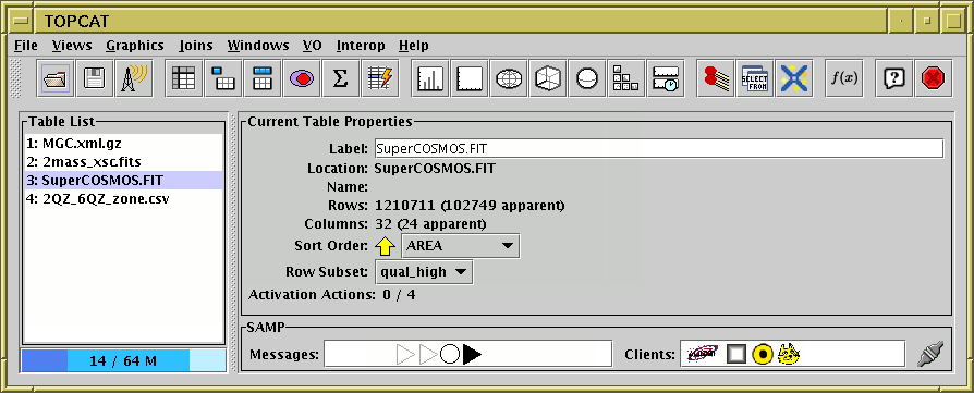
The main control window having loaded in some FITS and VOTable
files. The right hand panel describes the characteristics of the
current table, SuperCOSMOS.FIT.
The buttons along the top allow launching of various other windows.
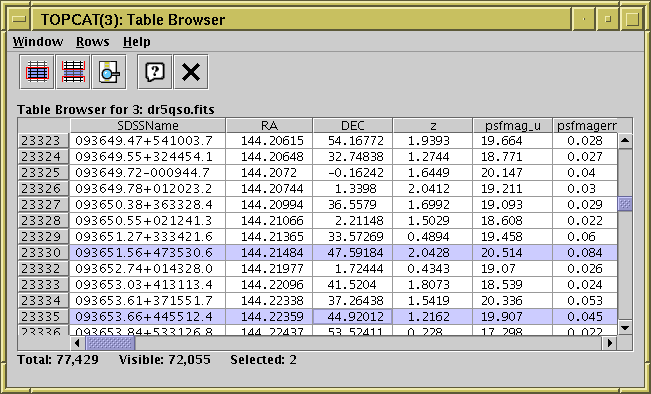
The data window shows the cells which constitute the table's data. It's easy to scroll around the rows and columns rapidly, even for very large tables. The rows displayed can be sorted, and some or all of the rows displayed.
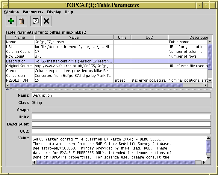
The parameters window displays some basic information about the table as well as stored per-table metadata. New parameters can be defined and saved.
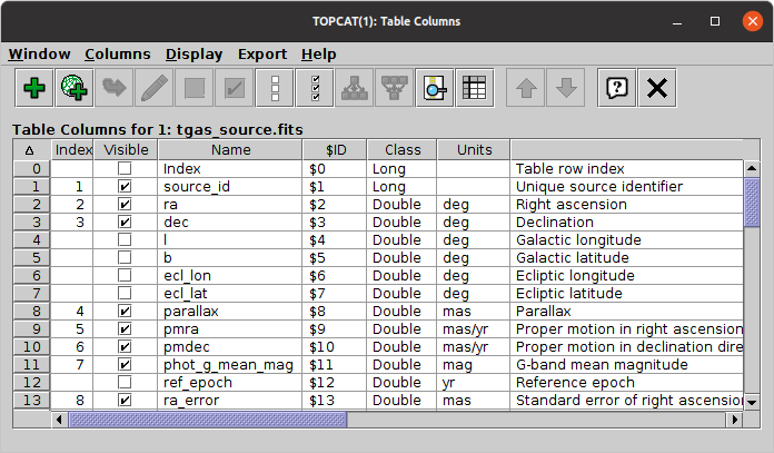
The columns window displays what is known about each column: name, units, type, shape, description UCD etc. Columns can be hidden/revealed, and new ones added.
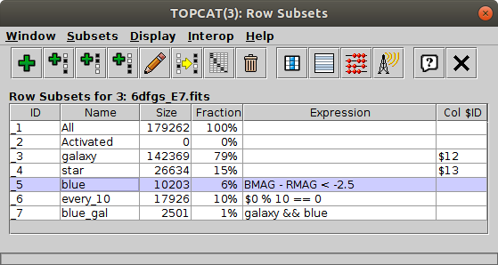
The subsets window allows you to see all the row subsets which have been defined, and to define more. Row subsets are selections of the rows in a table, and can be defined using a powerful algebraic expression language, or graphically from the plot window, or in other ways.
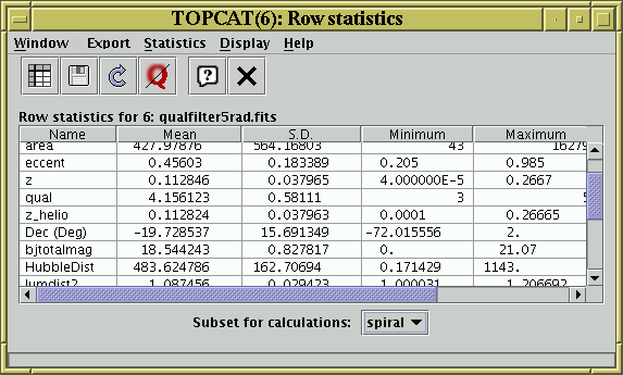
The statistics window allows you to calculate statistics for all or a selection of rows in the table. Various univariate quantities such as mean, variance, maximum, minimum, sum, number of good values etc are calculated and displayed for each of the columns.
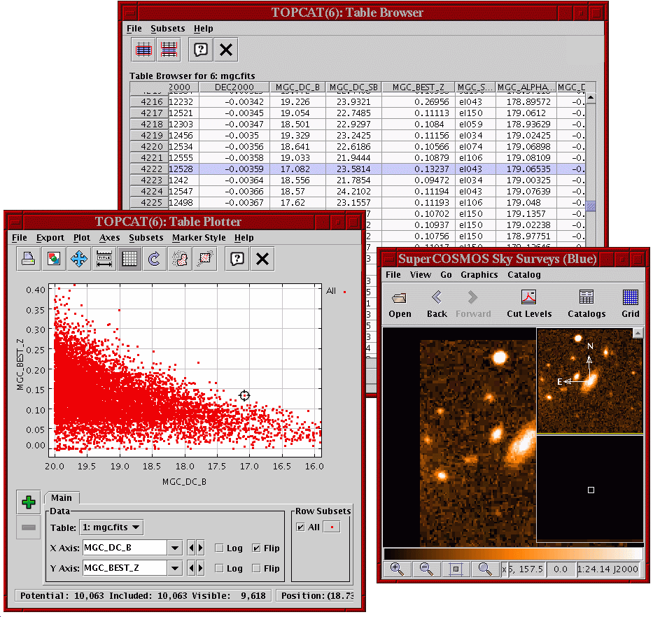
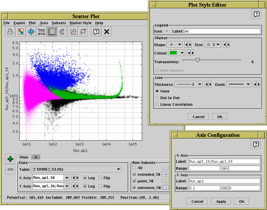
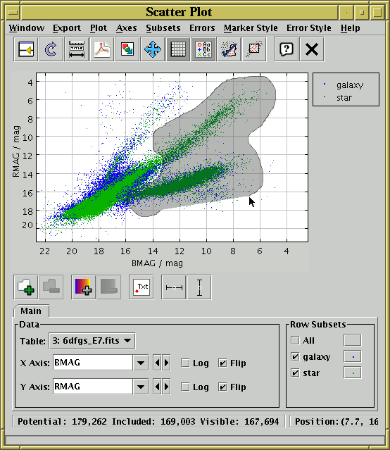
The plot window allows you to plot pairs of columns from one or more tables against each other. Points from different tables, columns or defined row subsets can be plotted using different colours or symbols. The dialogues to the upper right shows how you can configure the plot markers for the different datasets including symbol colour, shape, transparency (very useful for very crowded plots). You can zoom in or out easily using by dragging the mouse or by typing ranges into the dialogue shown at the lower right.
Within the plot window you can trace out a region with the mouse to define a new subset of points. This can be used in other contexts in the program, for instance calculating statistics on that set, matching points against it, or saving a table containing only those rows. This screenshot demonstrates tracing out a blob-shaped region corresponding to one branch of a magnitude-magnitude scatter plot.
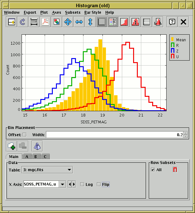
The other graphics windows, shown below, allow the same kinds of configuration as the 2D scatter plot.
Plots 1-d hisgtograms.
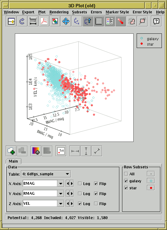
Plots 3D scatter plots on Cartesian axes. You can rotate the axes by dragging the mouse around on the window.
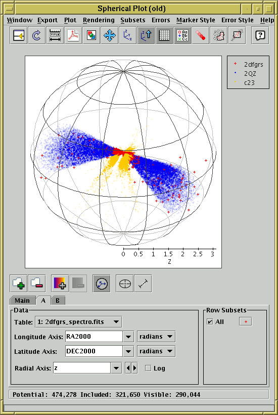
Plots 3D scatter plots on spherical polar axes. The radial coordinate is optional, so you can either plot points only on the surface of the sphere or on the interior. You can rotate the axes by dragging the mouse around on the window.
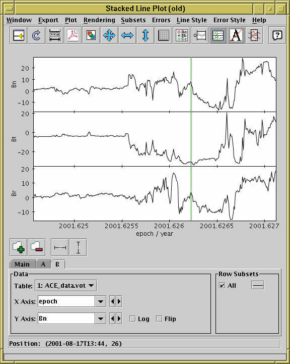
Plots one or more X-Y line plots using the same X axis but different Y axes. This can be particularly useful for visualising time-seres data.
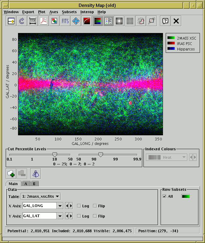
Plots a density map or, to look at it another way, a histogram on a 2-dimensional grid. The intensity of colour at each pixel reflects the number of points that fall within its bounds. Pixel size can be changed, cut levels can be altered, and the result can be exported to a FITS array for further analysis. This is very useful for analysis and visualisation of extremely crowded plots.
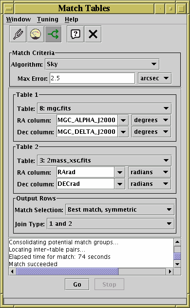
The match window allows you to specify a match operation which will join two tables. A wide range of multivariate matches is possible.
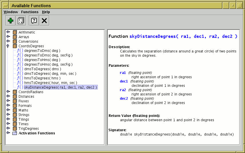
The available functions window displays the details of the functions which can be used within the algebraic expression language used to define new columns and subsets. The list of functions can be expanded at runtime with user-supplied java classes.
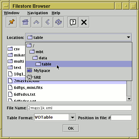
You can load tables from a number of sources. As well as a normal filesystem browser, there are facilities to acquire tables a number of other sources.
The default file browser looks much like a standard one, but also permits you to log into remote MySpace or SRB servers to access files using those protocols:
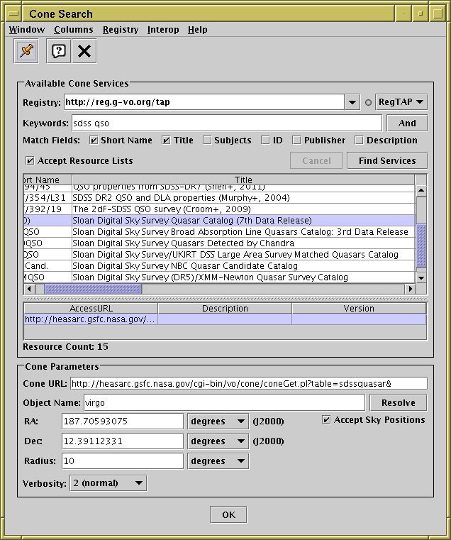
This dialogue displays a number of cone search services available on the web (the list is obtained from a VO registry) and allows you to interrogate them to find a catalogue of objects in a given region of the sky:
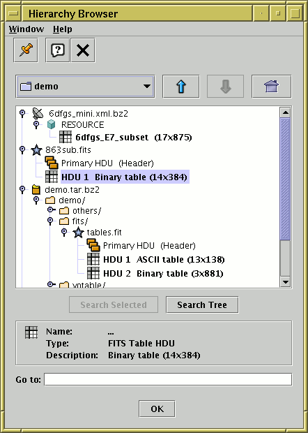
This one shows you a "Treeview"-like view of a filesystem, allowing you to poke around inside tar archives, FITS files and VOTable documents to find the table you're after:
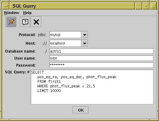
This one allows you to acquire a table by executing an SQL query on a local or remote relational database:
You can 'activate' a row either by clicking on its row in the data window, or by clicking on its point in a plot. In this case the data window row will be highlighted and the point will be marked with a visible cursor. Optionally, you can also configure some other action to take place when a point is activated, for instance display of a cutout from the sky corresponding to that row. This screenshot shows that happening.