Starlink User Note 256
Mark Taylor
14 May 2026
stilts command
cmd_*)
mode_*)
fits
colfits
votable
cdf
csv
ecsv
ascii
ipac
pds4
mrt
parquet
hapi
feather
gbin
tst
ver
wdc
fits
votable
csv
ecsv
ascii
ipac
parquet
feather
text
html
latex
tst
mirage
addcol
addpixsample
addresolve
addskycoords
assert
badval
cache
check
clearparams
collapsecols
colmeta
constcol
delcols
every
explodeall
explodecols
fixcolnames
group
head
healpixmeta
keepcols
meta
progress
random
randomview
repeat
replacecol
replaceval
rowrange
select
seqview
setparam
shuffle
sort
sorthead
stats
tablename
tail
transpose
uniq
sky: Sky Matching
skyerr:
Sky Matching with Per-Object Errors
skyellipse:
Sky Matching of Elliptical Regions
sky3d: Spherical Polar Matching
exact: Exact Matching
1d, 2d, ...:
Isotropic Cartesian Matching
2d_anisotropic, ...:
Anisotropic Cartesian Matching
2d_cuboid, ...:
Cuboid Cartesian Matching
1d_err, 2d_err, ...:
Cartesian Matching with Per-Object Errors
2d_ellipse:
Cartesian Matching of Elliptical Regions
mark
size
sizexy
xyvector
xyerror
xyellipse
xycorr
link2
mark2
poly4
mark4
polygon
area
central
lines
marks
handles
yerrors
xyerrors
statline
statmark
arrayquantile
line
linearfit
label
arealabel
contour
grid
fill
vecfield
quantile
histogram
kde
knn
densogram
gaussian
function
skyvector
skyellipse
skycorr
skydensity
skyvecfield
healpix
skygrid
xyzvector
xyzerror
line3d
spheregrid
yerror
spectrogram
auto
flat
translucent
transparent
density
aux
weighted
paux
pweighted
arrayjoin: Adds table-per-row data as array-valued columns
calc: Evaluates expressions
cdsskymatch:
Crossmatches table on sky position against VizieR/SIMBAD table
cone: Executes a Cone Search-like query
coneskymatch:
Crossmatches table on sky position against remote cone service
datalinklint:
Validates DataLink documents
doc: Displays STILTS documentation in a web browser
funcs: Browses functions used by algebraic expression language
mocshape: Generates Multi-Order Coverage maps from shape values
parqlint: Checks parquet file compliance with VOParquet convention
parqlook: Presents information about a parquet file
pixfoot: Generates Multi-Order Coverage maps
pixsample: Samples from a HEALPix pixel data file
plot2plane: Draws a plane plot
plot2sky: Draws a sky plot
plot2cube: Draws a cube plot
plot2sphere:
Draws a sphere plot
plot2corner: Draws a matrix of plane plots
plot2time: Draws a time plot
plot2d: Old-style 2D Scatter Plot
plot3d: Old-style 3D Scatter Plot
plothist: Old-style Histogram
regquery: Queries the VO registry
server: Runs an HTTP server to perform STILTS commands
sqlclient:
Executes SQL statements
sqlskymatch:
Crossmatches table on sky position against SQL table
sqlupdate: Updates values in an SQL table
taplint: Tests TAP services
tapquery: Queries a Table Access Protocol server
tapresume: Resumes a previous query to a Table Access Protocol server
tapskymatch:
Crossmatches table on sky position against TAP table
tcat: Concatenates multiple similar tables
tcatn: Concatenates multiple tables
tcopy: Converts between table formats
tcube: Calculates N-dimensional histograms
tloop: Generates a single-column table from a loop variable
tgridmap: Calculates N-dimensional density maps
tgroup: Calculates aggregate functions on groups of rows
tjoin: Joins multiple tables side-to-side
tmatch1: Performs a crossmatch internal to a single table
tmatch2: Crossmatches 2 tables using flexible criteria
tmatchn: Crossmatches multiple tables using flexible criteria
tmulti: Writes multiple tables to a single container file
tmultin: Writes multiple processed tables to single container file
tpipe: Performs pipeline processing on a table
tskymap: Calculates sky density maps
tskymatch2: Crossmatches 2 tables on sky position
votcopy: Transforms between VOTable encodings
votlint: Validates VOTable documents
xsdvalidate:
Validates against XML Schema
STILTS is a set of command-line tools for processing tabular data. It has been designed for, but is not restricted to, use on astronomical data such as source catalogues. It contains both generic (format-independent) table processing tools and tools for processing VOTable documents. Facilities offered include crossmatching, format conversion, format validation, column calculation and rearrangement, row selection, sorting, plotting, statistical calculations and metadata display. Calculations on cell data can be performed using a powerful and extensible expression language.
The package is written in pure Java (except for a few optional libraries) and based on STIL, the Starlink Tables Infrastructure Library. This gives it high portability, support for many data formats (including FITS, VOTable, text-based formats and SQL databases), extensibility and scalability. Where possible the tools are written to accept streamed data so the size of tables which can be processed is not limited by available memory. As well as the tutorial and reference information in this document, detailed on-line help is available from the tools themselves.
The STILTS application is available under the GNU General Public License (GPL) though most parts of the library code may alternatively be used under the GNU Lesser General Public License (LGPL).
STILTS provides a number of command-line applications which can be used for manipulating tabular data. Conceptually it sits between, and uses many of the same classes as, the packages STIL, which is a set of Java APIs providing table-related functionality, and TOPCAT, which is a graphical application providing the user with an interactive platform for exploring one or more tables. This document is mostly self-contained - it covers some of the same ground as the STIL and TOPCAT user documents (SUN/252 and SUN/253 respectively).
Currently, this package consists of commands in the following categories:
tcopy,
tpipe,
tmulti,
tmultin,
tcat,
tcatn,
tloop,
tjoin,
arrayjoin,
tgridmap,
tgroup, and
tcube
(see Section 6).
tmatch1,
tmatch2,
tmatchn and
tskymatch2
(see Section 7).
plot2plane,
plot2sky,
plot2cube,
plot2sphere,
plot2corner and
plot2time
(also deprecated old-style plot commands
plot2d,
plot3d and
plothist)
(see Section 8).
tskymap,
mocshape,
pixfoot and
pixsample.
votcopy and
votlint.
cdsskymatch,
cone,
coneskymatch,
tapquery,
tapresume,
tapskymatch,
taplint,
datalinklint and
regquery.
sqlclient,
sqlupdate and
sqlskymatch.
calc,
doc,
funcs,
parqlint,
parqlook,
server and
xsdvalidate.
There are many ways you might want to use these tools; here are a few possibilities:
server command may help,
but is not required, for use in these situations.
stilts command
All the functions available in this package can be used from
a single command, which is usually referred to in this document
simply as "stilts". Depending on how you have installed
the package, you may just type "stilts",
or something like
java -jar some/path/stilts.jaror
java -classpath topcat-full.jar uk.ac.starlink.ttools.Stiltsor something else - this is covered in detail in Section 3.
In general, the form of a command is
stilts <stilts-flags> <task-name> <task-args>The forms of the parts of this command are described in the following subsections, and details of each of the available tasks along with their arguments are listed in the command reference at the end of this document. Some of the commands are highly configurable and have a variety of parameters to define their operation. In many cases however, it's not complicated to use them. For instance, to convert the data in a FITS table to VOTable format you might write:
stilts tcopy cat.fits cat.vot
Some flags are common to all the tasks in the STILTS package,
and these are specified after the stilts invocation itself
and before the task name. They generally have the same effect
regardless of which task is running. These generic flags are as
follows:
-help
stilts command
itself and exits. The message contains a listing of all the
known tasks.
-version
-verbose
+verbose can be used to do the opposite
(reduce the logging level by one notch).
-allowunused
-prompt
-prompt flag,
then you will be prompted for every parameter you have not
explicitly specified to give you an opportunity to enter a value
other than the default.
-bench
-debug
-batch
-batch flag,
then you won't be prompted at all.
-memory
-Dstartable.storage=memory.
-disk
-Dstartable.storage=disk.
-memgui
-checkversion <vers>
<vers>. If it is not, STILTS will exit with
an error. This can be useful when executing in certain controlled
environments to ensure that the correct version of the application
is being picked up.
-stdout <file>
-" for <file>
will restore this default behaviour.
-stderr <file>
-" for <file>
will restore this default behaviour.
If you are submitting an error report, please include the result of
running stilts -version and the output of the troublesome
command with the -debug flag specified.
The <task-name> part of the command line is the
name of one of the tasks listed in Appendix B - currently
the available tasks are:
arrayjoin
calc
cdsskymatch
cone
coneskymatch
datalinklint
doc
funcs
mocshape
parqlint
parqlook
pixfoot
pixsample
plot2corner
plot2cube
plot2plane
plot2sphere
plot2sky
plot2time
plot2d
plot3d
plothist
regquery
server
sqlclient
sqlskymatch
sqlupdate
taplint
tapquery
tapresume
tapskymatch
tcat
tcatn
tcopy
tcube
tgridmap
tgroup
tjoin
tloop
tmatch1
tmatch2
tmatchn
tmulti
tmultin
tpipe
tskymap
tskymatch2
votcopy
votlint
xsdvalidate
The <task-args> part of the command line is a
list of parameter assignments,
each giving the value of one of the named parameters belonging to
the task which is specified in the <task-name> part.
The general form of each parameter assignment is
<param-name>=<param-value>If you want to set the parameter to the null value, which is legal for some but not all parameters, use the special string "
null",
or just leave the value blank ("<param-name>=").
In some cases you can optionally leave out the <param-name>
part of the assignment (i.e. the parameter is positionally determined);
this is indicated in the task's usage description if the parameter
is described like [<param-name>=]<param-value>
rather than <param-name>=<param-value>.
If the <param-value> contains spaces or other special
characters, then in most cases, such as from the Unix shell, you will
have to quote it somehow. How this is done depends on your platform,
but usually surrounding the whole value in single quotes will do the trick.
Tasks may have many parameters, and you don't have to set all of them explicitly on the comand line. For a parameter which you don't set, two things can happen. In many cases, it will default to some sensible value. Sometimes however, you may be prompted for the value to use. In the latter case, a line like this will be written to the terminal:
matcher - Name of matching algorithm [sky]:This is prompting you for the value of the parameter named
matcher. "Name of matching algorithm" is a short
description of what that parameter does. "sky" is
the default value (if there is no default, no value will appear
in square brackets).
At this point you can do one of four things:
null".null" means the null value,
which is legal for some, but not all parameters.
If the value you enter is not legal, you will see an error
message and you will be invited to try again. help" or a question mark "?".
This will output a message
giving a detailed description of the parameter
and prompt you again.stilts
command itself (see Section 2.1).
If you supply the -prompt flag, then you will be prompted
for every parameter you have not explicitly set. If you supply
-batch on the other hand, you won't be prompted for
any parameters (and if you fail to set any without legal default
values, the task will fail).
If you want to see the actual values of the parameters for a task
as it runs,
including prompted values and defaulted ones
which you haven't specified explicitly,
you can use the -verbose flag after the stilts
command:
   % stilts -verbose tcopy cat.fits cat.vot ifmt=fits
   INFO: tcopy in=cat.fits out=cat.vot ifmt=fits ofmt=(auto)
If you make a parameter assignment on the command line for a
parameter which is not used by the task in question, STILTS
will issue an error message and the task will fail.
Note some parameters are only used dependent on the presence or
values of other parameters, so even supplying a parameter which is
documented in the task's usage can have this effect.
This is done on the assumption that if you have supplied a spurious
parameter it's probably a mistake and you should be given the
opportunity to correct it.
But if you want to be free to make these mistakes without the
task failing, you can supply the -allowunused flag
as described in Section 2.1, in which case they will
just result in a warning.
Note that when running STILTS from the shell, it may be necessary to quote some parameter values, in case they contain spaces or other characters which the shell may try to interpret. This can typically be done by writing assignments of the form
<param-name>='<param-value>'but things can get more hairy; see Section 10.6 for more detail.
Extensive help is available from stilts
itself about task and its parameters, as described in the next section.
As well as the command descriptions in this document (especially the reference section Appendix B) you can get help for STILTS usage from the command itself. Typing
stilts -helpresults in this output:
   Usage:
      stilts [-help] [-version] [-verbose] [-allowunused] [-prompt] [-bench]
             [-debug] [-batch] [-memory] [-disk] [-memgui]
             [-checkversion <vers>] [-stdout <file>] [-stderr <file>]
             <task-name> <task-args>

      stilts <task-name> help[=<param-name>|*]

      Known tasks:
         arrayjoin
         calc
         cdsskymatch
         cone
         coneskymatch
         datalinklint
         doc
         funcs
         mocshape
         parqlint
         parqlook
         pixfoot
         pixsample
         plot2d
         plot3d
         plothist
         regquery
         server
         sqlclient
         sqlskymatch
         sqlupdate
         taplint
         tapquery
         tapresume
         tapskymatch
         tcat
         tcatn
         tcopy
         tcube
         tgridmap
         tgroup
         tjoin
         tloop
         tmatch1
         tmatch2
         tmatchn
         tmulti
         tmultin
         tpipe
         tskymap
         tskymatch2
         votcopy
         votlint
         xsdvalidate
         plot2plane
         plot2sky
         plot2cube
         plot2sphere
         plot2corner
         plot2time
For help on the individual tasks, including their parameter lists,
you can supply the word help
after the task name, so for instance
stilts tcopy helpresults in
   Usage: tcopy ifmt=<in-format> ofmt=<out-format>
                [in=]<table> [out=]<out-table>
Finally, you can get help on any of the parameters of a task
by writing help=<param-name>, like this:
stilts tcopy help=ingives
   Help for parameter IN in task TCOPY
   -----------------------------------

      Name:
         in

      Usage:
         [in=]<table>

      Summary:
         Location of input table

      Description:
         The location of the input table. This may take one of the following
         forms:

          * A filename.
          * A URL.
          * The special value "-", meaning standard input. In this case the
               input format must be given explicitly using the ifmt parameter.
               Note that not all formats can be streamed in this way.
          * A scheme specification of the form :<scheme-name>:<scheme-args>.
          * A system command line with either a "<" character at the start, or
               a "|" character at the end ("<syscmd" or "syscmd|"). This
               executes the given pipeline and reads from its standard output.
               This will probably only work on unix-like systems.

         In any case, compressed data in one of the supported compression
         formats (gzip, Unix compress or bzip2) will be decompressed
         transparently.

      Type:
         uk.ac.starlink.table.StarTable
If you use "*" instead of a parameter name in this usage,
help for all the parameters will be printed. Note that in most shells
you will probably need to quote the asterisk, so you should write
stilts tcopy help='*'
In some cases, as described in Section 2.3, you will be prompted for the value of a parameter with a line something like this:
matcher - Name of matching algorithm [sky]:In this case, if you enter "
help" or a question mark,
then the parameter help entry will be printed to the screen, and
the prompt will be repeated.
For more detailed descriptions of the tasks, which includes explanatory comments and examples as well as the information above, see the full task descriptions in the Command Reference.
There are a number of ways of invoking commands
in the stilts application,
depending on how you have installed the package.
This section describes how to invoke it from the command line.
Other options are using it from Jython (the Java implementation of
the Python language) as described in Section 4,
invoking it over HTTP as described in Section 11,
and invoking it from within a Java application
as described in Section 12.
If you're using a Unix-like operating system,
the easiest way is to use the stilts script.
It is a simple shell script which just invokes java with the
right classpath and the supplied arguments.
If you have a full starjava installation the stilts script
is in the starjava/bin directory.
Otherwise you can download it separately from wherever you got your
STILTS installation in the first place, or find it
at the top of the stilts.jar or topcat-*.jar file
that contains your STILTS installation, so do something like
   unzip stilts.jar stilts
   chmod +x stilts
to extract it (if you don't have
unzip,
try jar xvf stilts.jar stilts).
If you have mounted the topcat-all.dmg file on MacOS
(hdiutil attach topcat-all.dmg) it will probably be
present at a location like
/Volumes/topcat/TOPCAT.app/Contents/Resources/app/stilts.
To run using the stilts script, first make sure that
both the java
executable and the stilts script itself are on your path,
and that the stilts.jar or topcat-*.jar
jar file is in the same directory as stilts.
Then the form of invocation is:
stilts <java-flags> <stilts-flags> <task-name> <task-args>A simple example would be:
stilts votcopy format=binary t1.xml t2.xmlin this case, as often, there are no
<java-flags> or
<stilts-flags>.
If you use the -classpath
argument or have a CLASSPATH environment variable set,
then classpath elements thus specified will be added to the classpath
required to run the command.
The examples in the
command descriptions below use this form for convenience.
If you don't have a Unix-like shell available however,
you will need to invoke
Java directly with the appropriate classes on your classpath.
If you have the file stilts.jar, in most cases you can
just write:
java <java-flags> -jar stilts.jar <stilts-flags> <task-name> <task-args>which in practice would look something like
java -jar /some/where/stilts.jar votcopy format=binary t1.xml t2.xml
In the most general case, Java's -jar flag might be
no good, for one of the following reasons:
stilts.jar
file (such as topcat-full.jar)
   java <java-flags> -classpath <class-path>
        uk.ac.starlink.ttools.Stilts <stilts-flags> <task-name> <task-args>
The example above in this case would look something like:
   java -classpath /some/where/topcat-full.jar uk.ac.starlink.ttools.Stilts
        votcopy format=binary t1.xml t2.xml
Finally, as a convenience, it is possible to run STILTS from a
TOPCAT
installation by using its -stilts flag, like this:
topcat <java-flags> -stilts <stilts-flags> <task-name> <task-args>This is possible because TOPCAT is built on top of STILTS, so contains a superset of its code.
The
<stilts-flags>,
<task-name> and
<task-args>
parts of these invocations are explained in Section 2,
and the
<class-path> and
<java-flags>
parts are explained in the following subsections.
The classpath is the list of places that Java looks to find
the bits of compiled code that it uses to run an application.
Depending on how you have done your installation the core STILTS
classes could be in various places, but they are probably in a
file with one of the names
stilts.jar,
topcat-full.jar or
topcat-extra.jar.
The full pathname of one of these files can therefore be used as
your classpath. In some cases these files are self-contained and
in some cases they reference other jar files in the filesystem -
this means that they may or may not continue to work if you
move them from their original location.
Under certain circumstances the tools might need additional classes, for instance:
In most cases it is not necessary to specify any additional arguments to the Java runtime, but it can be useful in certain circumstances. The two main kinds of options you might want to specify directly to Java are these:
-Dname=value.
So for instance to ensure that temporary files are written to
the /home/scratch directory, you could use the flag
-Djava.io.tmpdir=/home/scratch
-Xmx flag. To set the heap
memory size to 256 megabytes, use the flag
-Xmx256M
(don't forget the 'M' for megabyte). You will probably find
performance is dreadful if you specify a heap size larger than
the physical memory of the machine you're running on.
You can specify other options to Java such as tuning and profiling flags etc, but if you want to do that sort of thing you probably don't need me to tell you about it.
If you are using the stilts command-line script,
any flags to it starting -D or -X are passed
directly to the java executable.
You can pass other flags to Java with the stilts script's
-J flag; for instance:
stilts -Xmx4M -J-verbose:gc calc 'mjdToIso(0)'is equivalent to
java -Xmx4M -verbose:gc -jar stilts.jar calc 'mjdToIso(0)'
System properties are a way of getting information into the
Java runtime - they are a bit like environment variables.
There are two ways to set them when using STILTS: either
on the command line using arguments of the form
-Dname=value (see Section 3.2)
or in a file in your home directory named
.starjava.properties, in the form of a
name=value line.
Thus submitting the flag
-Dvotable.strict=falseon the command line is equivalent to having the following in your
.starjava.properties file:
   #  Force strict interpretation of the VOTable standard.
   votable.strict=false
The following system properties have special significance to STILTS:
http.proxyHost
java.awt.headless
true" if running the
plotting tasks on a headless server.
You only need to worry about this if you see error messages
complaining about headlessness.
java.io.tmpdir
/tmp on Unix),
so if working with large unmapped (e.g. CSV) tables
on a machine with limited space on the default disk,
it may be necessary to change it.
java.util.concurrent.ForkJoinPool.common.parallelism
jdbc.drivers
jel.classes
mark.workaround
mark()/reset() methods of some java
InputStream classes. These are rather common,
including in Sun's J2SE system libraries.
Use this if you are seeing errors that say something like
"Resetting to invalid mark".
Currently defaults to "false".service.maxparallel
auth.username
auth.password
@<filename>",
in which case the value is read from the first line of the named file.
This replaces the normal behaviour of asking for a username and
password on the console; see the
section on Authentication
for more details.
Since this setting will pass the username and password information to any
protected resource without checking it is the intended destination,
this can potentially leak secret information to third parties,
so these properties should be set with care.
auth.schemes
AuthScheme
implementation classnames may be provided.
startable.readers
uk.ac.starlink.table.TableBuilder interface,
and must have a no-arg constructor.
The readers thus named will be available
alongside the standard ones listed in Section 5.1.1.
startable.schemes
uk.ac.starlink.table.TableScheme interface,
and must have a no-arg constructor.
The schemes thus named will be available
alongside the standard ones listed in Section 5.3.
startable.storage
disk" has basically the same effect as
supplying the "-disk" argument on the command line
(see Section 2.1).
Other possible values are "adaptive", "memory",
"sideways" and "discard";
see SUN/252.
The default is "adaptive", which means storing smaller
tables in memory, and larger ones on disk.
startable.unmap
sun" (the default),
"cleaner", "unsafe" or "none".
In most cases you are advised to leave this alone, but in the event of
unmapping-related JVM crashes (not expected!), setting it to
none may help.
startable.writers
uk.ac.starlink.table.StarTableWriter interface,
and must have a no-arg constructor.
The writers thus named will be available
alongside the standard ones listed in Section 5.1.2.
votable.namespacing
none" (no namespacing, xmlns declarations
in VOTable document will probably confuse parser),
"lax" (anything that looks like it is probably a VOTable
element will be treated as a VOTable element) and
"strict" (VOTable elements must be properly declared in one
of the correct VOTable namespaces).
May also be set to the classname of a
uk.ac.starlink.votable.Namespacing implementation.
The default is "lax".
votable.strict
FIELD or PARAM element with
a datatype attribute of
char/unicodeChar,
and no arraysize attribute.
The VOTable standard says this indicates a single character,
but some VOTables omit arraysize specification by accident when
they intend arraysize="*".
If votable.strict is set true,
a missing arraysize will be interpreted as meaning a single character,
and if false, it will be interpreted as a variable-length
array of characters (a string).
The default is true.
votable.version
1.0", "1.1",
"1.2", "1.3" or "1.4".
By default, version 1.4 VOTables are written.
This section describes additional configuration which must be done to allow the commands to access SQL-compatible relational databases for reading or writing tables. If you don't need to talk to SQL-type databases, you can ignore the rest of this section. The steps described here are the standard ones for configuring JDBC (which sort-of stands for Java Database Connectivity); you can find more information on that on the web. The best place to look may be within the documentation of the RDBMS you are using.
To use STILTS with SQL-compatible databases you must:
jdbc.drivers system property to the name of the
driver class as described in Section 3.3
Here is an example of using tpipe
to write the results
of an SQL query on a table in a MySQL database as a VOTable:
   stilts -classpath /usr/local/jars/mysql-connector-java.jar \
          -Djdbc.drivers=com.mysql.jdbc.Driver \
          tpipe \
          in="jdbc:mysql://localhost/db1#SELECT id, ra, dec FROM gsc WHERE mag < 9" \
          ofmt=votable gsc.vot
or invoking Java directly:
   java -classpath stilts.jar:/usr/local/jars/mysql-connect-java.jar \
        -Djdbc.drivers=com.mysql.jdbc.Driver \
        uk.ac.starlink.ttools.Stilts tpipe \
        in="jdbc:mysql://localhost/db1#SELECT id, ra, dec FROM gsc WHERE mag < 9" \
        ofmt=votable out=gsc.vot
You have to exercise some care to get the arguments
in the right order here - see Section 3.
Alternatively, you can set some of this up beforehand to make the invocation easier. If you set your CLASSPATH environment variable to include the driver jar file (and the STILTS classes if you're invoking Java directly rather than using the scripts), and if you put the line
jdbc.drivers=com.mysql.jdbc.Driverin the
.starjava.properties file in your home directory,
then you could avoid having to give the -classpath and
-Djdbc.drivers flags respectively.
Below are presented the results of some experiments with JDBC drivers. Note however that this information may be be incomplete and out of date. If you have updates, feel free to pass them on and they may be incorporated here.
To the author's knowledge, STILTS has successfully been used with the following RDBMSs and corresponding JDBC drivers:
useUnicode=true&characterEncoding=UTF8" may be required
to handle some non-ASCII characters.
jdbc:sybase:Tds:hostname:port/dbname?user=XXX&password=XXX#SELECT...".
An earlier attempt using Sybase ASE 11.9.2 failed.
Here are some example command lines that at least have at some point got STILTS running with databases:
   stilts -classpath pg73jdbc3.jar \
          -Djdbc.drivers=org.postgresql.Driver ...
   stilts -classpath mysql-connector-java-3.0.8-bin.jar \
          -Djdbc.drivers=com.mysql.jdbc.Driver ...
   stilts -classpath ojdbc14.jar \
          -Djdbc.drivers=oracle.jdbc.driver.OracleDriver ...
   stilts -classpath jtds-1.1.jar \
          -Djdbc.drivers=net.sourceforge.jtds.jdbc.Driver ...
Most of the discussions and examples in this document describe using STILTS as a standalone java application from the command line; in this case, scripting can be achieved by executing one STILTS command, followed by another, followed by another, perhaps controlled from a shell script, with intermediate results stored in files.
However, it is also possible to invoke STILTS commands from within the Jython environment. Jython is a pure-java implementation of the widely-used Python scripting language. Using Jython is almost exactly the same as using the more usual C-based Python, except that it is not possible to use extensions which use C code. This means that if you are familiar with Python programming, it is very easy to string STILTS commands together in Jython.
This approach has several advantages over the conventional command-line usage:
Usage from jython has syntax which is similar to command-line STILTS, but with a few changes. The following functions are defined by JyStilts:
tread, which reads a table from a
file or URL and turns it into a table object in jython
write which takes a table object and
writes it to file
cmd_head, cmd_select,
cmd_addcol)
mode_out, mode_meta,
mode_samp),
tmatch2, tcat, plot2sky)
help" command, however
for full documentation and examples you should refer to this document.
In JyStilts the input, processing, filtering and output are done in separate steps, unlike in command-line STILTS where they all have to be combined into a single line. This can make the flow of execution easier to follow. A typical sequence will involve:
tread functioncmd_* filter methodscmd_* filter methodsmode_* output modeswrite methodHere is an example command line invocation for crossmatching two tables:
stilts tskymatch2 in1=survey.fits \
	     icmd1='addskycoords fk4 fk5 RA1950 DEC1950 RA2000 DEC2000' \
	     in2=mycat.csv ifmt2=csv \
	     icmd2='select VMAG>18' \
	     ra1=ALPHA dec1=DELTA ra2=RA2000 dec2=DEC2000 \
	     error=10 join=2not1 \
	     out=matched.fits
and here is what it might look like in JyStilts:
>>> import stilts
>>> t1 = stilts.tread('survey.fits')
>>> t1 = t1.cmd_addskycoords(t1, 'fk4', 'fk5', 'RA1950', 'DEC1950', 'RA2000', 'DEC2000')
>>> t2 = stilts.tread('mycat.csv', 'csv')
>>> t2 = t2.cmd_select('VMAG>18')
>>> tm = stilts.tskymatch2(in1=t1, in2=t2, ra1='ALPHA', dec1='DELTA',
...                        error=10, join='2not1')
>>> tm.write('matched.fits')
When running interactively, it can be convenient to examine the intermediate results before processing or writing as well, for instance:
>>> tm.mode_count()
columns: 19   rows: 2102
>>> tm.cmd_keepcols('ID ALPHA DELTA').cmd_head(4).write()
+--------+---------------+-----------+
| ID     | ALPHA         | DELTA     |
+--------+---------------+-----------+
| 262    | 149.82439     | -0.11249  |
| 263    | 150.14438     | -0.11785  |
| 265    | 149.92944     | -0.11667  |
| 273    | 149.93185     | -0.12566  |
+--------+---------------+-----------+
More detail about how to run JyStilts and its usage is given in the following subsections.
The easiest way to run JyStilts is to download the standalone
jystilts.jar file from the STILTS web page,
and simply run
java -jar jystilts.jarThis file includes jython itself and all the STILTS and JyStilts classes. To use the JyStilts commands, you will need to import the stilts module using a line like "
import stilts"
from Jython in the usual Python way.
Alternatively, you can run JyStilts from an existing Jython installation
using just the stilts.jar file.
First, make sure that Jython is installed;
it is available from http://www.jython.org/,
and comes as a self-installing jar file.
JyStilts has been tested, and appears to work, with jython version 2.7.2.
It also works with jython 2.5.* under Java 8 and Java 11,
but jystilts with jython 2.5.* and Java 17 can fail with security problems.
Some earlier versions of JyStilts worked with jython 2.2.1,
but that no longer seems to be the case; it might be possible
to reinstate this if there is some pressing need.
To use JyStilts, you then just need to
start jython with the stilts.jar file on your classpath,
for instance like this:
jython -J-classpath /some/where/stilts.jaror (C-shell):
setenv CLASSPATH /some/where/stilts.jar
jython
Optionally, you can extract the stilts.py module
from the stilts.jar file
(using a command like "unzip stilts.jar stilts.py")
and put it in a directory on your jython
sys.path (e.g. jythondir/Lib);
this may cause jython to compile it to bytecode (stilts$py.class)
and thus improve startup time.
Note that in this case you will still need the stilts.jar
file on your classpath as above.
The tread function reads tables from an external location
into JyStilts. Its arguments are as follows:
tread(location, fmt='(auto)', random=False)and its return value is a table object, which can be interrogated directly, or used in other JyStilts commands. Usually, the location argument should be a string which gives the filename or URL at which a table can be found. You can alternatively use a readable python file (or file-like) object for the location, but be aware that this may be less efficient on memory. As with command-line STILTS, the
fmt argument
is one of the options in Section 5.1.1, but may be
left as the default if the format auto-detectable,
which currently means if the file is in
VOTable, FITS, CDF, ECSV, PDS4, Parquet, Feather or GBIN format.
The random argument can be used to ensure that the returned file
has random (i.e. not sequential-only) access;
for some table formats the default way of reading them in means that
their rows can only be accessed in sequence.
Depending on what processing you are doing, that may or may not be
satisfactory.
Examples of reading a table are:
>>> import stilts
>>> t1 = stilts.tread('cat.fits')
>>> t2 = stilts.tread(open('cat.fits', 'rb'))           # less efficient
>>> t3 = stilts.tread('data.csv', fmt='csv', random=True)
The most straightforward way to write a table
(presumably the result of one or a sequence of JyStilts commands)
is using the write table method:
write(self, location=None, fmt='(auto)')The
location gives either a string which is a filename,
or a writable python file (or file-like) object.
Again, use of a filename is preferred as it may(?) be more efficient.
If no location is supplied, the table will be written to standard output
(useful for inspection, but a bad idea for binary formats or very large tables).
The fmt argument is one of the output formats in
Section 5.1.2, but may be left as the default if the
format can be guessed from the filename.
Examples of writing a table are:
>>> table.write('out.fits')
>>> table.write(open('out.fits', 'wb'))       #  less efficient?
>>> table.write('catalogue.dat', fmt='csv')
>>> table.write()                             #  display to stdout
Often it's convenient to combine examining the table with filtering steps, for instance:
>>> table.every(100).write()would write only every hundredth row, and
>>> (table.cmd_sorthead(10, 'BMAG')
...       .cmd_select('!NULL_VMAG')
...       .cmd_keepcols('BMAG VMAG')
...       .write())
would write only the BMAG and VMAG columns
for the ten rows in which VMAG is non-null with the lowest BMAG values.
You can also read and write multiple tables, if you use a table
format for which that is appropriate.
This generally means FITS (which can store tables in multiple extensions)
or VOTable (which can store multiple TABLE elements in one document).
This is done using the treads and twrites functions.
The functions look like this:
treads(location, fmt='(auto)', random=False)
twrites(tables, location=None, fmt='(auto)')
These are similar to the
tread and twrite functions,
except that treads returns a list of tables rather than
a single table, and twrites's tables argument is
an iterable over tables rather than a single table.
Here is an example of reading multiple tables from a multi-extension FITS
file, counting the rows in each, and then writing them out to a multi-TABLE
VOTable file:
import stilts
tables = stilts.treads('multi.fits')
print([t.getRowCount() for t in tables])
stilts.twrites(tables, 'multi.vot', fmt='votable')
The tables read by the tread function and produced
by operating on them within JyStilts have a number of methods
defined on them.
These are explained below.
First, a number of special methods are defined which allow a table to behave in python like a sequence of rows:
__iter__
for row in table:" will iterate over all rows.
__len__ (random-access tables only)
len(table)" to count the number of rows.
This method is not available for tables with sequential access only.
__getitem__ (random-access tables only)
table[3]" or table[0:10] to obtain the
row or rows corresponding to a given row index or slice.
This method is not available for tables with sequential access only.
__add__, __mul__, __rmul__
+" and and "*" to be used with
the sense of concatenation.
Thus "table1+table2" will produce a new table with the
rows of table1 followed by the rows of table2.
Note this will only work if both tables have compatible columns.
Similarly "table*3" would produce a table like
table but with all its rows repeated three times.
columns().
Sometimes, the result of a table operation will be a table which
does not have random access. For such tables you can iterate over
the rows, but not get their row values by indexing.
Non-random-access tables are also peculiar in that getRowCount
returns a negative value.
To take a table which may not have random access and make it capable
of random access, use the random
filter: "table=table.cmd_random()".
To a large extent it is possible to duplicate the functions of the
various STILTS commands by writing your own python code based on these
python-friendly table access methods.
Note however that such python-based processing is likely to be
much slower than the STILTS equivalents.
If performance is important to you, you should try in most cases
to use the various cmd_* commands etc for table processing.
Second, some additional utility methods are defined:
count_rows()
columns()
getName(),
getUnitString(), getUCD().
str(column) will return its name.
coldata(key)
key argument may be either an integer
column index (if negative, counts backwards from the end),
or the column name or info object.
The returned value will always be iterable (has __iter__),
but will only be indexable
(has __len__ and __getitem__) if the table
is random access.
parameters()
StarTable methods.
Note that as currently implemented, changing the values in the
returned mapping will not change the actual table parameter values.
write(location=None, fmt=None)
location argument gives a filename
or writable file object,
and the optional fmt argument gives a format, one of
the options listed in Section 5.1.1.
If location is not supplied, output is to standard output,
so in an interactive session it will be printed to the terminal.
If fmt is not supplied, an attempt will be made to guess
a suitable format based on the location.
Third, a set of cmd_* methods corresponding to the
STILTS filters are available;
these are described in Section 4.4.
Fourth, a set of mode_* methods corresponding to the
STILTS output modes are available;
these are described in Section 4.5.
Finally, tables are also instances of the StarTable interface defined by STIL, which is the table I/O layer underlying STILTS. The full documentation can be found in the user manual and javadocs on the STIL page, and all the java methods can be used from JyStilts, but in most cases there are more pythonic equivalents provided, as described above.
Here are some examples of these methods in use:
   >>> import stilts
   >>> xsc = stilts.tread('/data/table/2mass_xsc.xml')  # read table
   >>> xsc.mode_count()                                 # show rows/column count
   columns: 6   rows: 1646844
   >>> print xsc.columns()                              # full info on columns
   (id(String), ra(Double)/degrees, dec(Double)/degrees, jmag(Double)/mag, hmag(Double)/mag, kmag(Double)/mag)
   >>> print [str(col) for col in xsc.columns()]        # column names only
   ['id', 'ra', 'dec', 'jmag', 'hmag', 'kmag']
   >>> row = xsc[1000000]                               # examine millionth row
   >>> print row
   (u'19433000+4003190', 295.875, 40.055286, 14.449, 13.906, 13.374)
   >>> print row[0]                                     # cell by index
   19433000+4003190
   >>> print row['ra'], row['dec']                      # cells by col name
   295.875 40.055286
   >>> print len(xsc)                                   # count rows, maybe slow
   1646844
   >>> print xsc.count_rows()                           # count rows efficiently
   1646844L
   >>> print (xsc+xsc).count_rows()                     # concatenate
   3293688L
   >>> print (xsc*10000).count_rows()
   16468440000L
   >>> for row in xsc:                  # select rows using python commands
   ...     if row[4] - row[3] > 3.0:
   ...         print row[0]
   ...
   11165243+2925509
   20491597+5119089
   04330238+0858101
   01182715-1013248
   11244075+5218078
   >>>                                  # same thing using stilts (50x faster)
   >>> (xsc.cmd_select('hmag - jmag > 3.0')
   ...     .cmd_keepcols('id')
   ...     .write())
   +------------------+
   | id               |
   +------------------+
   | 11165243+2925509 |
   | 20491597+5119089 |
   | 04330238+0858101 |
   | 01182715-1013248 |
   | 11244075+5218078 |
   +------------------+
The following are all ways to obtain the value of a given cell in the table from the previous example.
    xsc.getCell(99, 0)
    xsc[99][0]
    xsc[99]['id']
    xsc.coldata(0)[99]
    xsc.coldata('id')[99]
Some of these methods may be more efficient than others.
Note that none of these methods will work if the table has sequential-only
access.
cmd_*)
The STILTS table filters documented in Section 6.1
are available in JyStilts as table methods
which start with the "cmd_" prefix.
The return value when calling the method on a table object is
another table object.
The arguments, which are the same as those required for the command-line
version, are supplied as a list of unnamed arguments of the
cmd_* function. In general the arguments are strings,
but numbers are accepted where appropriate.
Use the python help command to see the usage of each method.
So, to use the tail filter to
select only the last ten lines of a table, you can write:
table.cmd_tail(10)To set units of "Hz" for some columns using the
colmeta filter write:
table.cmd_colmeta('-units', 'Hz', 'AFREQ BFREQ CFREQ')
Note that where a filter argument is a space-separated list
it must appear as a single argument in the filter invocation,
just as in command-line STILTS.
The filter commands are also available as module functions. This means that
stilts.cmd_head(table, 10)and
table.cmd_head(10)have exactly the same meaning. It's a matter of taste which you prefer.
mode_*)
The STILTS table output modes documented in Section 6.4
are available in JyStilts as table methods
which start with the "mode_" prefix.
These methods have no return value, but cause something to happen,
in some cases output to be written to standard output.
Some of these methods have named arguments, others have no arguments.
Use the python help command to see the usage of each method.
These methods are straightforward to use. The following example calculates statistics for a table and writes the results to standard output:
>>> table.mode_stats()and this one attempts to send the table via the SAMP communications protocol to a running instance of TOPCAT:
>>> table.mode_samp(client='topcat')
The output modes are also available as module functions. This means that
stilts.mode_samp(table, client='topcat')and
table.mode_samp(client='topcat)have exactly the same meaning. It's a matter of taste which you prefer.
The STILTS tasks documented in Appendix B
can be used under their usual names if they are imported from the
stilts module.
STILTS parameters as are supplied as named arguments of the python
functions. In general they are either table objects for table input
parameters or strings, but in some cases python arrays are accepted,
and numbers may be used where appropriate.
The STILTS input format (ifmt, istream),
filter (cmd/icmd/ocmd)
and output mode (omode) parameters are not used however;
instead perform filtering directly on the table inputs and outputs
using the python cmd_* and mode_*
table methods or functions.
Here is an example of concatenating two similar tables together and writing the result:
   >>> from stilts import tread, tcat
   >>> t1 = tread('data1.csv', fmt='csv')
   >>> t2 = tread('data2.csv', fmt='csv')
   >>> t12 = tcat([t1,t2], seqcol='seq')
   >>> t12.write('t12.csv', fmt='csv')
Note that for those tasks which have a parameter named "in"
in command-line STILTS, it has been renamed as "in_" for
the python version, to avoid a name clash with the python reserved word.
In most cases, the in parameter is the first, mandatory
parameter in any case, and so can be referenced by position as in the
previous example (we could have written "tcat(in_=[t1,t2])"
instead).
The various functions from the expression language
listed in Section 10.7 are available directly from JyStilts.
Each of the subsections in that section is a class in the stilts
module namespace, with unbound functions representing the functions.
This means you can use them like this:
    >>> import stilts
    >>> print stilts.Times.mjdToIso(54292)
    2007-07-11T00:00:00
or like this:
    >>> from stilts import CoordsDegrees
    >>> dist = CoordsDegrees.skyDistanceDegrees(ra1, dec1, ra2, dec2)
Most of the tools in this package either read one or more tables as input, or write one or more tables as output, or both. This section explains what kind of tables the tools can read and write, and how you tell them where to find the tables to operate on.
In most cases input and output table specifications are given by parameters with the following names (or similar ones):
in
ifmt
out
-"/blank for standard output
ofmt
The generic table commands in STILTS
(currently tpipe,
tcopy,
tmulti,
tmultin,
tcat,
tcatn,
tloop,
tjoin,
tgridmap,
tgroup,
tcube,
tmatch1,
tmatch2,
tmatchn,
tskymap,
tskymatch2,
pixfoot,
pixsample,
plot2corner,
plot2cube,
plot2plane,
plot2sky,
plot2sphere,
plot2time,
plot2d,
plot3d,
plothist,
cdsskymatch,
cone,
coneskymatch,
sqlskymatch,
tapquery,
tapresume,
tapskymatch and
regquery)
have no native format for table storage, they can process
data in a number of formats equally well.
STIL has its own model of what a table
consists of, which is basically:
The formats the package knows about are dependent on the input and output handlers currently installed. The ones installed by default are listed in the following subsections. More may be added in the future, and it is possible to install new ones at runtime - see the STIL documentation for details.
Some formats can be used to hold multiple tables in a single file, and others can only hold a single table per file.
Some of the tools in this package ask you to specify the format
of input tables using the ifmt (or a similarly named)
parameter.
For some file formats (e.g. FITS, VOTable, CDF),
the format can be automatically determined by
looking at the file content, regardless of filename;
for others (e.g. CSV files with a ".csv" extension),
STILTS may be able to use the filename as a hint to guess the format
(the details of these rules are given in the format-specific
subsections below).
Otherwise, you have to supply the format using the ifmt parameter.
It is always safe to specify the format explicitly;
this will be slightly more efficient than auto-determination,
and may lead to more helpful error messages in the case that the
table can't be read correctly.
The available input formats are described in the following subsections.
It is also possible to add new formats at runtime using the
startable.readers system property,
or by setting the format to the classname of a
uk.ac.starlink.table.TableBuilder class.
fits
FITS is a very well-established format for storage of
astronomical table or image data
(see https://fits.gsfc.nasa.gov/).
This reader can read tables stored in
binary (XTENSION='BINTABLE') and
ASCII (XTENSION='TABLE') table extensions;
any image data is ignored.
Currently, binary table extensions are read much more efficiently
than ASCII ones.
When a table is stored in a BINTABLE extension in an uncompressed FITS file on disk, the table is 'mapped' into memory; this generally means very fast loading and low memory usage. FITS tables are thus usually efficient to use.
Limited support is provided for the semi-standard HEALPix-FITS convention; such information about HEALPix level and coordinate system is read and made available for application usage and user examination.
A private convention is used to support encoding of tables with more than 999 columns (not possible in standard FITS); see Section 5.1.3.2.
Header cards in the table's HDU header will be made available as table parameters. Only header cards which are not used to specify the table format itself are visible as parameters (e.g. NAXIS, TTYPE* etc cards are not). HISTORY and COMMENT cards are run together as one multi-line value.
Any 64-bit integer column with a non-zero integer offset
(TFORMn='K', TSCALn=1, TZEROn<>0)
is represented in the read table as Strings giving the decimal integer value,
since no numeric type in Java is capable of representing the whole range of
possible inputs. Such columns are most commonly seen representing
unsigned long values.
Where a multi-extension FITS file contains more than one table, a single table may be specified using the position indicator, which may take one of the following forms:
spec23.fits.gz"
with one primary HDU and two BINTABLE extensions,
you would view the first one using the name "spec23.fits.gz"
or "spec23.fits.gz#1"
and the second one using the name "spec23.fits.gz#2".
The suffix "#0" is never used for a legal
FITS file, since the primary HDU cannot contain a table.
EXTNAME header in the HDU,
or alternatively the value of EXTNAME
followed by "-" followed by the value of EXTVER.
This follows the recommendation in
the FITS standard that EXTNAME and EXTVER
headers can be used to identify an HDU.
So in a multi-extension FITS file "cat.fits"
where a table extension
has EXTNAME='UV_DATA' and EXTVER=3,
it could be referenced as
"cat.fits#UV_DATA" or "cat.fits#UV_DATA-3".
Matching of these names is case-insensitive.
Files in this format may contain multiple tables;
depending on the context, either one or all tables
will be read.
Where only one table is required,
either the first one in the file is used,
or the required one can be specified after the
"#" character at the end of the filename.
This format can be automatically identified by its content so you do not need to specify the format explicitly when reading FITS tables, regardless of the filename.
There are actually two FITS input handlers,
fits-basic and fits-plus.
The fits-basic handler extracts standard column metadata
from FITS headers of the HDU in which the table is found,
while the fits-plus handler reads column and table metadata
from VOTable content stored in the primary HDU of the multi-extension
FITS file.
FITS-plus is a private convention effectively defined by the
corresponding output handler; it allows de/serialization of
much richer metadata than can be stored in standard FITS headers
when the FITS file is read by fits-plus-aware readers,
though other readers can understand the unenhanced FITS file perfectly well.
It is normally not necessary to worry about this distinction;
STILTS will determine whether a FITS file is FITS-plus or not based on its
content and use the appropriate handler, but if you want to force the
reader to use or ignore the enriched header, you can explicitly specify
an input format of "fits-plus" or "fits-basic".
The details of the FITS-plus convention are described in Section 5.1.3.1.
colfits
As well as normal binary and ASCII FITS tables, STIL supports
FITS files which contain tabular data stored in column-oriented format.
This means that the table is stored in a BINTABLE extension HDU,
but that BINTABLE has a single row, with each cell of that row
holding a whole column's worth of data. The final (slowest-varying)
dimension of each of these cells (declared via the TDIMn headers)
is the same for every column, namely,
the number of rows in the table that is represented.
The point of this is that all the cells for each column are stored
contiguously, which for very large, and especially very wide tables
means that certain access patterns (basically, ones which access
only a small proportion of the columns in a table) can be much more
efficient since they require less I/O overhead in reading data blocks.
Such tables are perfectly legal FITS files, but general-purpose FITS software may not recognise them as multi-row tables in the usual way. This format is mostly intended for the case where you have a large table in some other format (possibly the result of an SQL query) and you wish to cache it in a way which can be read efficiently by a STIL-based application.
For performance reasons, it is advisable to access colfits files uncompressed on disk. Reading them from a remote URL, or in gzipped form, may be rather slow (in earlier versions it was not supported at all).
This format can be automatically identified by its content so you do not need to specify the format explicitly when reading colfits-basic tables, regardless of the filename.
Like the normal (row-oriented) FITS handler,
two variants are supported:
with (colfits-plus) or without (colfits-basic)
metadata stored as a VOTable byte array in the primary HDU.
For details of the FITS-plus convention, see Section 5.1.3.1.
votable
VOTable is an XML-based format for tabular data endorsed by the International Virtual Observatory Alliance; while the tabular data which can be encoded is by design close to what FITS allows, it provides for much richer encoding of structure and metadata. Most of the table data exchanged by VO services is in VOTable format, and it can be used for local table storage as well.
Any table which conforms to the VOTable 1.0, 1.1, 1.2, 1.3 or 1.4 specifications can be read. This includes all the defined cell data serializations; cell data may be included in-line as XML elements (TABLEDATA serialization), included/referenced as a FITS table (FITS serialization), or included/referenced as a raw binary stream (BINARY or BINARY2 serialization). The handler does not attempt to be fussy about input VOTable documents, and it will have a good go at reading VOTables which violate the standards in various ways.
Much, but not all, of the metadata contained in a VOTable
document is retained when the table is read in.
The attributes
unit, ucd, xtype and utype,
and the elements
COOSYS, TIMESYS and DESCRIPTION
attached to table columns or parameters,
are read and may be used by the application as appropriate
or examined by the user.
However, information encoded in the hierarchical structure
of the VOTable document, including GROUP structure, is not
currently retained when a VOTable is read.
VOTable documents may contain more than one actual table
(TABLE element).
To specify a specific single table,
the table position indicator is given by the
zero-based index of the TABLE element in a breadth-first search.
Here is an example VOTable document:
   <VOTABLE>
     <RESOURCE>
       <TABLE name="Star Catalogue"> ... </TABLE>
       <TABLE name="Galaxy Catalogue"> ... </TABLE>
     </RESOURCE>
   </VOTABLE>
If this is available in a file named "cats.xml"
then the two tables could be named as
"cats.xml#0" and "cats.xml#1" respectively.
Files in this format may contain multiple tables;
depending on the context, either one or all tables
will be read.
Where only one table is required,
either the first one in the file is used,
or the required one can be specified after the
"#" character at the end of the filename.
This format can be automatically identified by its content so you do not need to specify the format explicitly when reading VOTable tables, regardless of the filename.
cdf
NASA's Common Data Format, described at https://cdf.gsfc.nasa.gov/, is a binary format for storing self-described data. It is typically used to store tabular data for subject areas like space and solar physics.
CDF does not store tables as such, but sets of variables
(columns) which are typically linked to a time quantity;
there may be multiple such disjoint sets in a single CDF file.
This reader attempts to extract these sets into separate tables
using, where present, the DEPEND_0 attribute
defined by the
ISTP Metadata Guidelines.
Where there are multiple tables they can be identified
using a "#" symbol at the end of the filename
by index ("<file>.cdf#0" is the first table)
or by the name of the independent variable
("<file>.cdf#EPOCH" is the table relating to
the EPOCH column).
Files in this format may contain multiple tables;
depending on the context, either one or all tables
will be read.
Where only one table is required,
either the first one in the file is used,
or the required one can be specified after the
"#" character at the end of the filename.
This format can be automatically identified by its content so you do not need to specify the format explicitly when reading CDF tables, regardless of the filename.
csv
Comma-separated value ("CSV") format is a common semi-standard text-based format in which fields are delimited by commas. Spreadsheets and databases are often able to export data in some variant of it. The intention is to read tables in the version of the format spoken by MS Excel amongst other applications, though the documentation on which it was based was not obtained directly from Microsoft.
The rules for data which it understands are as follows:
#" character
(or anything else) to introduce "comment" lines.
Because the CSV format contains no metadata beyond column names,
the handler is forced to guess the datatype of the values in each column.
It does this by reading the whole file through once and guessing
on the basis of what it has seen (though see the maxSample
configuration option). This has the disadvantages:
The delimiter option makes it possible to use non-comma
characters to separate fields. Depending on the character used this
may behave in surprising ways; in particular for space-separated fields
the ascii format may be a better choice.
The handler behaviour may be modified by specifying
one or more comma-separated name=value configuration options
in parentheses after the handler name, e.g.
"csv(header=true,delimiter=|)".
The following options are available:
header = true|false|null
true: the first line is a header line containing column namesfalse: all lines are data lines, and column names will be assigned automaticallynull: a guess will be made about whether the first line is a header or not depending on what it looks likenull (auto-determination).
This usually works OK, but can get into trouble if
all the columns look like string values.
(Default: null)
delimiter = <char>|0xNN
|", a hexadecimal character code like "0x7C", or one of the names "comma", "space" or "tab". Some choices of delimiter, for instance whitespace characters, might not work well or might behave in surprising ways.
(Default: ,)
maxSample = <int>
0)
notypes = <type>[;<type>...]
blank, boolean, short, int, long, float, double, date, hms and dms. So if you want to make sure that all integer and floating-point columns are 64-bit (i.e. long and double respectively) you can set this value to "short;int;float".encoding = ASCII|UTF-8|UTF-16|...
UTF-8)
This format cannot be automatically identified
by its content, so in general it is necessary
to specify that a table is in
CSV
format when reading it.
However, if the input file has
the extension ".csv" (case insensitive)
an attempt will be made to read it using this format.
An example looks like this:
RECNO,SPECIES,NAME,LEGS,HEIGHT,MAMMAL
1,pig,Pigling Bland,4,0.8,true
2,cow,Daisy,4,2.0,true
3,goldfish,Dobbin,,0.05,false
4,ant,,6,0.001,false
5,ant,,6,0.001,false
6,queen ant,Ma'am,6,0.002,false
7,human,Mark,2,1.8,true
See also ECSV as a format which is similar and capable of storing more metadata.
ecsv
The Enhanced Character Separated Values format was developed within the Astropy project and is described in Astropy APE6 (DOI). It is composed of a YAML header followed by a CSV-like body, and is intended to be a human-readable and maybe even human-writable format with rich metadata. Most of the useful per-column and per-table metadata is preserved when de/serializing to this format. The version supported by this reader is currently ECSV 1.0.
There are various ways to format the YAML header, but a simple example of an ECSV file looks like this:
# %ECSV 1.0
# ---
# delimiter: ','
# datatype: [
#   { name: index,   datatype: int32   },
#   { name: Species, datatype: string  },
#   { name: Name,    datatype: string  },
#   { name: Legs,    datatype: int32   },
#   { name: Height,  datatype: float64, unit: m },
#   { name: Mammal,  datatype: bool    },
# ]
index,Species,Name,Legs,Height,Mammal
1,pig,Bland,4,,True
2,cow,Daisy,4,2,True
3,goldfish,Dobbin,,0.05,False
4,ant,,6,0.001,False
5,ant,,6,0.001,False
6,human,Mark,2,1.9,True
If you follow this pattern, it's possible to write your own ECSV files by
taking an existing CSV file
and decorating it with a header that gives column datatypes,
and possibly other metadata such as units.
This allows you to force the datatype of given columns
(the CSV reader guesses datatype based on content, but can get it wrong)
and it can also be read much more efficiently than a CSV file
and its format can be detected automatically.
The header information can be provided either in the ECSV file itself,
or alongside a plain CSV file from a separate source
referenced using the header configuration option.
In Gaia EDR3 for instance, the ECSV headers are supplied alongside
the CSV files available for raw download of all tables in the
Gaia source catalogue, so e.g. STILTS can read
one of the gaia_source CSV files with full metadata
as follows:
   stilts tpipe
      ifmt='ecsv(header=http://cdn.gea.esac.esa.int/Gaia/gedr3/ECSV_headers/gaia_source.header)'
      in=http://cdn.gea.esac.esa.int/Gaia/gedr3/gaia_source/GaiaSource_000000-003111.csv.gz
The ECSV datatypes that work well with this reader are
bool,
int8, int16, int32, int64,
float32, float64
and
string.
Array-valued columns are also supported with some restrictions.
Following the ECSV 1.0 specification,
columns representing arrays of the supported datatypes can be read,
as columns with datatype: string and a suitable
subtype, e.g.
"int32[<dims>]" or "float64[<dims>]".
Fixed-length arrays (e.g. subtype: int32[3,10])
and 1-dimensional variable-length arrays
(e.g. subtype: float64[null]) are supported;
however variable-length arrays with more than one dimension
(e.g. subtype: int32[4,null]) cannot be represented,
and are read in as string values.
Null elements of array-valued cells are not supported;
they are read as NaNs for floating point data, and as zero/false for
integer/boolean data.
ECSV 1.0, required to work with array-valued columns,
is supported by Astropy v4.3 and later.
The handler behaviour may be modified by specifying
one or more comma-separated name=value configuration options
in parentheses after the handler name, e.g.
"ecsv(header=http://cdn.gea.esac.esa.int/Gaia/gedr3/ECSV_headers/gaia_source.header,colcheck=FAIL)".
The following options are available:
header = <filename-or-url>
null)
colcheck = IGNORE|WARN|FAIL
WARN)
This format can be automatically identified by its content so you do not need to specify the format explicitly when reading ECSV tables, regardless of the filename.
ascii
In many cases tables are stored in some sort of unstructured plain text format, with cells separated by spaces or some other delimiters. There is a wide variety of such formats depending on what delimiters are used, how columns are identified, whether blank values are permitted and so on. It is impossible to cope with them all, but the ASCII handler attempts to make a good guess about how to interpret a given ASCII file as a table, which in many cases is successful. In particular, if you just have columns of numbers separated by something that looks like spaces, you should be just fine.
Despite the name, by default it reads Unicode characters in the UTF-8
encoding. It can if necessary be restricted to ASCII characters only
by setting the encoding option.
Here are the detailed rules for how the ASCII-format tables are interpreted:
null" (unquoted) represents
the null valueBoolean,
Short
Integer,
Long,
Float,
Double,
String
NaN for not-a-number, which is treated the same as a
null value for most purposes, and Infinity or inf
for infinity (with or without a preceding +/- sign).
These values are matched case-insensitively.If the list of rules above looks frightening, don't worry, in many cases it ought to make sense of a table without you having to read the small print. Here is an example of a suitable ASCII-format table:
    #
    # Here is a list of some animals.
    #
    # RECNO  SPECIES         NAME         LEGS   HEIGHT/m
      1      pig             "Pigling Bland"  4  0.8
      2      cow             Daisy        4      2
      3      goldfish        Dobbin       ""     0.05
      4      ant             ""           6      0.001
      5      ant             ""           6      0.001
      6      ant             ''           6      0.001
      7      "queen ant"     'Ma\'am'     6      2e-3
      8      human           "Mark"       2      1.8
In this case it will identify the following columns:
    Name       Type
    ----       ----
    RECNO      Short
    SPECIES    String
    NAME       String
    LEGS       Short
    HEIGHT/m   Float
It will also use the text "Here is a list of some animals"
as the Description parameter of the table.
Without any of the comment lines, it would still interpret the table,
but the columns would be given the names col1..col5.
The handler behaviour may be modified by specifying
one or more comma-separated name=value configuration options
in parentheses after the handler name, e.g.
"ascii(maxSample=100000,notypes=short;float)".
The following options are available:
maxSample = <int>
0)
notypes = <type>[;<type>...]
blank, boolean, short, int, long, float, double, date, hms and dms. So if you want to make sure that all integer and floating-point columns are 64-bit (i.e. long and double respectively) you can set this value to "short;int;float".encoding = ASCII|UTF-8|UTF-16|...
UTF-8)
This format cannot be automatically identified
by its content, so in general it is necessary
to specify that a table is in
ASCII
format when reading it.
However, if the input file has
the extension ".txt" (case insensitive)
an attempt will be made to read it using this format.
ipac
CalTech's Infrared Processing and Analysis Center use a text-based format for storage of tabular data, defined at http://irsa.ipac.caltech.edu/applications/DDGEN/Doc/ipac_tbl.html. Tables can store column name, type, units and null values, as well as table parameters.
This format cannot be automatically identified
by its content, so in general it is necessary
to specify that a table is in
IPAC
format when reading it.
However, if the input file has
the extension ".tbl" or ".ipac" (case insensitive)
an attempt will be made to read it using this format.
An example looks like this:
\Table name = "animals.vot"
\Description = "Some animals"
\Author = "Mark Taylor"
| RECNO | SPECIES   | NAME          | LEGS | HEIGHT | MAMMAL |
| int   | char      | char          | int  | double | char   |
|       |           |               |      | m      |        |
| null  | null      | null          | null | null   | null   |
  1       pig         Pigling Bland   4      0.8      true
  2       cow         Daisy           4      2.0      true
  3       goldfish    Dobbin          null   0.05     false
  4       ant         null            6      0.001    false
  5       ant         null            6      0.001    false
  6       queen ant   Ma'am           6      0.002    false
  7       human       Mark            2      1.8      true
pds4
NASA's Planetary Data System version 4 format is described at https://pds.nasa.gov/datastandards/. This implementation is based on v1.16.0 of PDS4.
PDS4 files consist of an XML Label file which
provides detailed metadata, and which may also contain references
to external data files stored alongside it.
This input handler looks for (binary, character or delimited)
tables in the Label;
depending on the configuration it may restrict them to those
in the File_Area_Observational area.
The Label is the file which has to be presented to this
input handler to read the table data.
Because of the relationship between the label and the data files,
it is usually necessary to move them around together.
If there are multiple tables in the label,
you can refer to an individual one using the "#"
specifier after the label file name by table name,
local_identifier, or 1-based index
(e.g. "label.xml#1" refers to the first table).
If there are Special_Constants defined
in the label, they are in most cases interpreted as blank values
in the output table data.
At present, the following special values are interpreted
as blanks:
saturated_constant,
missing_constant,
error_constant,
invalid_constant,
unknown_constant,
not_applicable_constant,
high_instrument_saturation,
high_representation_saturation,
low_instrument_saturation,
low_representation_saturation
.
Fields within top-level Groups are interpreted as array values. Any fields in nested groups are ignored. For these array values only limited null-value substitution can be done (since array elements are primitives and so cannot take null values).
This input handler is somewhat experimental, and the author is not a PDS expert. If it behaves strangely or you have suggestions for how it could work better, please contact the author.
The handler behaviour may be modified by specifying
one or more comma-separated name=value configuration options
in parentheses after the handler name, e.g.
"pds4(checkmagic=false,observational=true)".
The following options are available:
checkmagic = true|false
true)
observational = true|false
<File_Area_Observational> element
of the PDS4 label should be included.
If true, only observational tables are found,
if false, other tables will be found as well.
(Default: false)
Files in this format may contain multiple tables;
depending on the context, either one or all tables
will be read.
Where only one table is required,
either the first one in the file is used,
or the required one can be specified after the
"#" character at the end of the filename.
This format can be automatically identified by its content so you do not need to specify the format explicitly when reading PDS4 tables, regardless of the filename.
mrt
The so-called "Machine-Readable Table" format is used by AAS journals, and based on the format of readMe files used by the CDS. There is some documentation at https://journals.aas.org/mrt-standards/, which mostly builds on documentation at https://vizier.cds.unistra.fr/doc/catstd.htx, but the format is in fact quite poorly specified, so this input handler was largely developed on a best-efforts basis by looking at MRT tables actually in use by AAS, and with assistance from AAS staff. As such, it's not guaranteed to succeed in reading all MRT files out there, but it will try its best.
It only attempts to read MRT files themselves, there is currently no capability to read VizieR data tables which provide the header and formatted data in separate files; however, if a table is present in VizieR, there will be options to download it in more widely used formats that can be used instead.
An example looks like this:
Title: A search for multi-planet systems with TESS using a Bayesian
       N-body retrieval and machine learning
Author: Pearson K.A.
Table: Stellar Parameters
================================================================================
Byte-by-byte Description of file: ajab4e1ct2_mrt.txt
--------------------------------------------------------------------------------
   Bytes Format Units   Label   Explanations
--------------------------------------------------------------------------------
   1-  9 I9     ---     ID      TESS Input Catalog identifier
  11- 15 F5.2   mag     Tmag    Apparent TESS band magnitude
  17- 21 F5.3   solRad  R*      Stellar radius
  23- 26 I4     K       Teff    Effective temperature
  28- 32 F5.3   [cm/s2] log(g)  log surface gravity
  34- 38 F5.2   [Sun]   [Fe/H]  Metallicity
  40- 44 F5.3   ---     u1      Linear Limb Darkening
  46- 50 F5.3   ---     u2      Quadratic Limb Darkening
--------------------------------------------------------------------------------
231663901 12.35 0.860 5600 4.489  0.00 0.439 0.138
149603524  9.72 1.280 6280 4.321  0.24 0.409 0.140
336732616 11.46 1.400 6351 4.229  0.00 0.398 0.140
231670397  9.85 2.070 6036 3.934  0.00 0.438 0.117
...
The handler behaviour may be modified by specifying
one or more comma-separated name=value configuration options
in parentheses after the handler name, e.g.
"mrt(errmode=FAIL,usefloat=true)".
The following options are available:
errmode = IGNORE|WARN|FAIL
warn)
usefloat = true|false
If it is set true,
then encountering values outside the representable range
will be reported in accordance with the current ErrorMode.
(Default: false)
checkmagic = true|false
Title: ".
Setting this true is generally a good idea
to avoid attempting to parse non-MRT files,
but you can set it false to attempt to read an MRT file
that starts with the wrong sequence.
(Default: true)
This format can be automatically identified by its content so you do not need to specify the format explicitly when reading MRT tables, regardless of the filename.
parquet
Parquet is a columnar format developed within the Apache project. Data is compressed on disk and read into memory before use. The file format is described at https://github.com/apache/parquet-format. This software is written with reference to version 2.10.0 of the format.
This input handler will read columns representing scalars, strings and one-dimensional arrays of the same. It is not capable of reading multi-dimensional arrays, more complex nested data structures, or some more exotic data types like 96-bit integers. If such columns are encountered in an input file, a warning will be emitted through the logging system and the column will not appear in the read table. Support may be introduced for some additional types if there is demand.
Parquet files typically do not contain rich metadata
such as column units, descriptions, UCDs etc.
To remedy that, this reader supports the
VOParquet convention (version 1.0),
in which metadata is recorded in a DATA-less VOTable
stored in the parquet file header.
If such metadata is present it will by default be used,
though this can be controlled using the votmeta
configuration option below.
Depending on the way that the table is accessed, the reader tries to take advantage of the column and row block structure of parquet files to read the data in parallel where possible.
Note:
The parquet I/O handlers require large external libraries, which are not always bundled with the library/application software because of their size. In some configurations, parquet support may not be present, and attempts to read or write parquet files will result in a message like:Parquet-mr libraries not availableIf you can supply the relevant libaries on the classpath at runtime, the parquet support will work. At time of writing, the required libraries are included in thetopcat-extra.jarmonolithic jar file (though nottopcat-full.jar), and are included if you have thetopcat-all.dmgfile. They can also be found in the starjava github repository (https://github.com/Starlink/starjava/tree/master/parquet/src/lib or you can acquire them from the Parquet MR package. These arrangements may be revised in future releases, for instance if parquet usage becomes more mainstream. The required dependencies are a minimal subset of those required by the Parquet MR submoduleparquet-cliat version 1.13.1, in particular the filesaircompressor-0.21.jarcommons-collections-3.2.2.jarcommons-configuration2-2.1.1.jarcommons-lang3-3.9.jarfailureaccess-1.0.1.jarguava-27.0.1-jre.jarhadoop-auth-3.2.3.jarhadoop-common-3.2.3.jarhadoop-mapreduce-client-core-3.2.3.jarhtrace-core4-4.1.0-incubating.jarparquet-cli-1.13.1.jarparquet-column-1.13.1.jarparquet-common-1.13.1.jarparquet-encoding-1.13.1.jarparquet-format-structures-1.13.1.jarparquet-hadoop-1.13.1.jarparquet-jackson-1.13.1.jarslf4j-api-1.7.22.jarslf4j-nop-1.7.22.jarsnappy-java-1.1.8.3.jarstax2-api-4.2.1.jarwoodstox-core-5.3.0.jarzstd-jni-1.5.0-1.jar.
These libraries support some, but not all, of the compression formats defined for parquet, currentlyuncompressed,gzip,snappy,zstdandlz4_raw. Supplying more of the parquet-mr dependencies at runtime would extend this list. Unlike the rest of TOPCAT/STILTS/STIL which is written in pure java, some of these libraries (currently the snappy and zstd compression codecs) contain native code, which means they may not work on all architectures. At time of writing all common architectures are covered, but there is the possibility of failure with ajava.lang.UnsatisfiedLinkErroron other platforms if attempting to read/write files that use those compression algorithms.
Note also that there are known problems with Parquet I/O when running with Java versions later than Java 21; you may encounter a message likejava.lang.UnsupportedOperationException: getSubject is not supportedThis is to do with the underlying Hadoop libraries (see this Hadoop bugtracking issue) and for now the only solution is to run using an earlier Java version like Java 8, 11, 17 or 21.
The handler behaviour may be modified by specifying
one or more comma-separated name=value configuration options
in parentheses after the handler name, e.g.
"parquet(cachecols=true,nThread=4)".
The following options are available:
cachecols = true|false|null
true, then when the table is loaded,
all data is read by column into local scratch disk files,
which is generally the fastest way to ingest all the data.
If false, the table rows are read as required,
and possibly cached using the normal STIL mechanisms.
If null (the default), the decision is taken
automatically based on available information.
(Default: null)
nThread = <int>
cachecols option.
If the value is <=0 (the default), a value is chosen
based on the number of apparently available processors.
(Default: 0)
tryUrl = true|false
false)
votmeta = true|false|null
IVOA.VOTable-Parquet.content
will be read to supply the metadata for the input table,
following the
VOParquet convention.
If false, any such VOTable metadata is ignored.
If set null, the default, then such VOTable metadata
will be used only if it is present and apparently consistent
with the parquet data and metadata.
(Default: null)
votable = <filename-or-url>
votmeta
configuration is not false.
(Default: null)
This format can be automatically identified by its content so you do not need to specify the format explicitly when reading parquet tables, regardless of the filename.
hapi
HAPI, the
Heliophysics Data Application Programmer's Interface
is a protocol for serving streamed time series data.
This reader can read HAPI CSV and binary tables
if they include header information
(the include=header request parameter
must be present).
An example HAPI URL is
https://vires.services/hapi/data?dataset=GRACE_A_MAG&start=2009-01-01&stop=2009-01-02&include=header
While HAPI data is normally accessed directly from the service, it is possible to download a HAPI stream to a local file and use this handler to read it from disk.
This format cannot be automatically identified
by its content, so in general it is necessary
to specify that a table is in
HAPI
format when reading it.
However, if the input file has
the extension ".hapi" (case insensitive)
an attempt will be made to read it using this format.
feather
The Feather file format is a column-oriented binary disk-based format based on Apache Arrow and supported by (at least) Python, R and Julia. Some description of it is available at https://github.com/wesm/feather and https://blog.rstudio.com/2016/03/29/feather/. It can be used for large datasets, but it does not support array-valued columns. It can be a useful format to use for exchanging data with R, for which FITS I/O is reported to be slow.
At present CATEGORY type columns are not supported, and metadata associated with TIME, DATE and TIMESTAMP columns is not retrieved.
This format can be automatically identified by its content so you do not need to specify the format explicitly when reading feather tables, regardless of the filename.
gbin
GBIN format is a special-interest file format used within DPAC, the Data Processing and Analysis Consortium working on data from the Gaia astrometry satellite. It is based on java serialization, and in all of its various forms has the peculiarity that you only stand any chance of decoding it if you have the Gaia data model classes on your java classpath at runtime. Since the set of relevant classes is very large, and also depends on what version of the data model your GBIN file corresponds to, those classes will not be packaged with this software, so some additional setup is required to read GBIN files.
As well as the data model classes, you must provide on the runtime classpath the GaiaTools classes required for GBIN reading. The table input handler accesses these by reflection, to avoid an additional large library dependency for a rather niche requirement. It is likely that since you have to supply the required data model classes you will also have the required GaiaTools classes to hand as well, so this shouldn't constitute much of an additional burden for usage.
In practice, if you have a jar file or files for pretty much any
java library or application which is capable of reading a given
GBIN file, just adding it or them to the classpath at runtime
when using this input handler ought to do the trick.
Examples of such jar files are
the
MDBExplorerStandalone.jar
file available from
https://gaia.esac.esa.int/mdbexp/,
or the gbcat.jar file you can build from the
CU9/software/gbcat/
directory in the DPAC subversion repository.
The GBIN format doesn't really store tables, it stores arrays of java objects, so the input handler has to make some decisions about how to flatten these into table rows.
In its simplest form, the handler basically looks for public instance
methods of the form getXxx()
and uses the Xxx as column names.
If the corresponding values are themselves objects with suitable getter
methods, those objects are added as new columns instead.
This more or less follows the practice of the gbcat
(gaia.cu1.tools.util.GbinInterogator) tool.
Method names are sorted alphabetically.
Arrays of complex objects are not handled well,
and various other things may trip it up.
See the source code (e.g. uk.ac.starlink.gbin.GbinTableProfile)
for more details.
If the object types stored in the GBIN file are known to the
special metadata-bearing class
gaia.cu9.tools.documentationexport.MetadataReader
and its dependencies, and if that class is on the runtime classpath,
then the handler will be able to extract additional metadata as available,
including standardised column names,
table and column descriptions, and UCDs.
An example of a jar file containing this metadata class alongside
data model classes is GaiaDataLibs-18.3.1-r515078.jar.
Note however at time of writing there are some deficiencies with this
metadata extraction functionality related to unresolved issues
in the upstream gaia class libraries and the relevant
interface control document
(GAIA-C9-SP-UB-XL-034-01, "External Data Centres ICD").
Currently columns appear in the output table in a more or less
random order, units and Utypes are not extracted,
and using the GBIN reader tends to cause a 700kbyte file "temp.xml"
to be written in the current directory.
If the upstream issues are fixed, this behaviour may improve.
Note: support for GBIN files is somewhat experimental. Please contact the author (who is not a GBIN expert) if it doesn't seem to be working properly or you think it should do things differently.
Note: there is a known bug in some versions of
GaiaTools (caused by a bug in its dependency library zStd-jni)
which in rare cases can fail to read all the rows in a GBIN input file.
If this bug is encountered by the reader, it will by default
fail with an error mentioning zStd-jni.
In this case, the best thing to do is to put a fixed version of zStd-jni
or GaiaTools on the classpath.
However, if instead you set the config option readMeta=false
the read will complete without error, though the missing rows will not
be recovered.
The handler behaviour may be modified by specifying
one or more comma-separated name=value configuration options
in parentheses after the handler name, e.g.
"gbin(readMeta=false,hierarchicalNames=true)".
The following options are available:
readMeta = true|false
Setting this false can prevent failing on an error related to a broken version of the zStd-jni library in GaiaTools.
Note however that in this case the data read, though not reporting an error, will silently be missing some rows from the GBIN file.
(Default: true)
hierarchicalNames = true|false
Astrometry_Alpha", if false they may just be called "Alpha".
In case of name duplication however, the hierarchical form is always used.
(Default: false)
This format can be automatically identified by its content so you do not need to specify the format explicitly when reading GBIN tables, regardless of the filename.
Example:
Suppose you have the MDBExplorerStandalone.jar file
containing the data model classes, you can read GBIN files by
starting STILTS like this:
stilts -classpath MDBExplorerStandalone.jar ...or like this:
java -classpath stilts.jar:MDBExplorerStandalone.jar uk.ac.starlink.ttools.Stilts ...
tst
Tab-Separated Table, or TST, is a text-based table format used
by a number of astronomical tools including Starlink's
GAIA
and
ESO's SkyCat
on which it is based.
A definition of the format can be found in
Starlink Software Note 75.
The implementation here ignores all comment lines: special comments
such as the "#column-units:" are not processed.
An example looks like this:
    Simple TST example; stellar photometry catalogue.

    A.C. Davenhall (Edinburgh) 26/7/00.

    Catalogue of U,B,V colours.
    UBV photometry from Mount Pumpkin Observatory,
    see Sage, Rosemary and Thyme (1988).

    # Start of parameter definitions.
    EQUINOX: J2000.0
    EPOCH: J1996.35

    id_col: -1
    ra_col: 0
    dec_col: 1

    # End of parameter definitions.
    ra<tab>dec<tab>V<tab>B_V<tab>U_B
    --<tab>---<tab>-<tab>---<tab>---
    5:09:08.7<tab> -8:45:15<tab>  4.27<tab>  -0.19<tab>  -0.90
    5:07:50.9<tab> -5:05:11<tab>  2.79<tab>  +0.13<tab>  +0.10
    5:01:26.3<tab> -7:10:26<tab>  4.81<tab>  -0.19<tab>  -0.74
    5:17:36.3<tab> -6:50:40<tab>  3.60<tab>  -0.11<tab>  -0.47
    [EOD]
This format cannot be automatically identified by its content, so in general it is necessary to specify that a table is in TST format when reading it.
ver
WARNING: this functionality and implementation is EXPERIMENTAL. Behaviour may change in future releases.
The Ver input handler is intended for reading tables in the loosely-defined "ver" format. This is a family of more or less ad-hoc(?) ASCII-based formats for specifying the shapes of 3d bodies.
There are usually two parts to such files, which are read by this handler as two tables: a list of 3d vertices, and a list of polygons referencing these vertices. The first line contains two integers, for the vertex and face counts.
At present, the vertices are represented as 3 columns X,Y,Z,
and the plates must be triangular and are represented as an intial
3-element position followed by a 6-element array of "other" positions.
This is just because those are in the form that's easy to plot
using the polygon layer type.
But there might be better ways to do this.
This implementation is hacky and includes behaviour to accommodate examples I've come across, mainly because I don't have a robust definition of the format(s). It may be improved in future, especially if a reliable definition of the format can be identified.
Some examples of files that this reader is able to read are:
Other resources:
Files in this format may contain multiple tables;
depending on the context, either one or all tables
will be read.
Where only one table is required,
either the first one in the file is used,
or the required one can be specified after the
"#" character at the end of the filename.
This format cannot be automatically identified
by its content, so in general it is necessary
to specify that a table is in
ver
format when reading it.
However, if the input file has
the extension ".ver" (case insensitive)
an attempt will be made to read it using this format.
wdc
Some support is provided for files produced by the World Data Centre for Solar Terrestrial Physics. The format itself apparently has no name, but files in this format look something like the following:
  Column formats and units - (Fixed format columns which are single space separated.)
  ------------------------
  Datetime (YYYY mm dd HHMMSS)            %4d %2d %2d %6d      -
                                          %1s
  aa index - 3-HOURLY (Provisional)       %3d                  nT

  2000 01 01 000000  67
  2000 01 01 030000  32
      ...
Support for this (obsolete?) format may not be very complete or robust.
This format cannot be automatically identified by its content, so in general it is necessary to specify that a table is in WDC format when reading it.
Some of the tools ask you to specify the format of output tables
using the ofmt parameter.
The output formats described below are supported; in some cases there
are variants or options for the basic formats as documented.
If you don't specify an output format explicitly,
STILTS will try to guess what format to write based on the
output filename; the details of those rules are also documented below.
It is also possible to add new formats at runtime using the
startable.writers system property,
or by setting the format to the classname of a
uk.ac.starlink.table.StarTableWriter class.
fits
FITS is a very well-established format for storage of astronomical table or image data (see https://fits.gsfc.nasa.gov/). This writer stores tables in BINTABLE extensions of a FITS file.
There are a number of variations in exactly how the table data is
written to FITS.
These can be configured with name=value options in brackets
as described below, but for most purposes this isn't required;
you can just choose fits or one of the standard
aliases for commonly-used combinations like colfits
or fits-basic.
In all cases the output from this handler is legal FITS, but some non-standard conventions are used:
primary=votable option or fits-plus alias
(if you don't want it,
use primary=basic or fits-basic).
This convention is described in more detail in Section 5.1.3.1.
col=true option or the colfits-plus/colfits-basic
aliases.
If you write to a file with the ".colfits" extension
it is used by default.
For convenience, and compatibility with earlier versions, these standard aliases are provided:
fits or fits(primary=votable).
fits(primary=basic).
fits(primary=basic,var=true).
fits(col=true).
fits(col=true,primary=basic).
fits-basic,
but it will rearrange and rename columns as required to follow
the convention, and it will fail if the table does not contain
the required HEALPix metadata (STIL_HPX_* parameters).
The handler behaviour may be modified by specifying
one or more comma-separated name=value configuration options
in parentheses after the handler name, e.g.
"fits(primary=basic,col=false)".
The following options are available:
primary = basic|votable[n.n]|none
basic
votable[n.n]
[n.n]" part
is optional, but if included
(e.g. "votable1.5")
indicates the version of the VOTable format to use.
none
votable)
col = true|false
false)
var = FALSE|TRUE|P|Q
True stores variable-length array values
after the main part of the table in the heap,
while false stores all arrays as fixed-length
(with a length equal to that of the longest array
in the column) in the body of the table.The options P or Q can be used
to force 32-bit or 64-bit pointers for indexing into the heap,
but it's not usually necessary since a suitable choice
is otherwise made from the data.
(Default: FALSE)
date = true|false
true)
Multiple tables may be written to a single output file using this format.
If no output format is explicitly chosen,
writing to a filename with
the extension ".fits", ".fit" or ".fts" (case insensitive)
will select fits format for output.
votable
VOTable is an XML-based format for tabular data endorsed by the International Virtual Observatory Alliance and defined in the VOTable Recommendation. While the tabular data which can be encoded is by design close to what FITS allows, it provides for much richer encoding of structure and metadata. Most of the table data exchanged by VO services is in VOTable format, but it can be used for local table storage as well.
When a table is saved to VOTable format, a document conforming to the
VOTable specification containing a single TABLE element within
a single RESOURCE element is written.
Where the table contains such information
(often obtained by reading an input VOTable),
column and table metadata will be written out as appropriate to
the attributes
unit, ucd, xtype and utype,
and the elements
COOSYS, TIMESYS and DESCRIPTION
attached to table columns or parameters.
There are various ways that a VOTable can be written;
by default the output serialization format is TABLEDATA
and the VOTable format version is 1.4, or a value controlled
by the votable.version system property.
However, configuration options are available to adjust these defaults.
The handler behaviour may be modified by specifying
one or more comma-separated name=value configuration options
in parentheses after the handler name, e.g.
"votable(format=BINARY2,version=1.3)".
The following options are available:
format = TABLEDATA|BINARY|BINARY2|FITS
TABLEDATA)
version = 1.0|1.1|1.2|1.3|1.4|1.5|1.6
1.3 may alternatively be written as V13 etc.
(Default: 1.4)
inline = true|false
true)
compact = true|false|null
null)
encoding = UTF-8|UTF-16|...
UTF-8)
date = true|false
true)
Multiple tables may be written to a single output file using this format.
If no output format is explicitly chosen,
writing to a filename with
the extension ".vot", ".votable" or ".xml" (case insensitive)
will select votable format for output.
csv
Writes tables in the semi-standard Comma-Separated Values format. This does not preserve any metadata apart from column names, and is generally inefficient to read, but it can be useful for importing into certain external applications, such as some databases or spreadsheets.
By default, the first line is a header line giving the column names,
but this can be inhibited using the header=false
configuration option.
The delimiter option makes it possible to use non-comma
characters to separate fields. Depending on the character used this
may behave in surprising ways; in particular for space-separated fields
the ascii format may be a better choice.
The handler behaviour may be modified by specifying
one or more comma-separated name=value configuration options
in parentheses after the handler name, e.g.
"csv(header=true,delimiter=|)".
The following options are available:
header = true|false
true)
delimiter = <char>|0xNN
|", a hexadecimal character code like "0x7C", or one of the names "comma", "space" or "tab". Some choices of delimiter, for instance whitespace characters, might not work well or might behave in surprising ways.
(Default: ,)
maxCell = <int>
2147483647)
encoding = ASCII|UTF-8|UTF-16|...
UTF-8)
If no output format is explicitly chosen,
writing to a filename with
the extension ".csv" (case insensitive)
will select CSV format for output.
An example looks like this:
RECNO,SPECIES,NAME,LEGS,HEIGHT,MAMMAL
1,pig,Pigling Bland,4,0.8,true
2,cow,Daisy,4,2.0,true
3,goldfish,Dobbin,,0.05,false
4,ant,,6,0.001,false
5,ant,,6,0.001,false
6,queen ant,Ma'am,6,0.002,false
7,human,Mark,2,1.8,true
ecsv
The Enhanced Character Separated Values format was developed within the Astropy project and is described in Astropy APE6 (DOI). It is composed of a YAML header followed by a CSV-like body, and is intended to be a human-readable and maybe even human-writable format with rich metadata. Most of the useful per-column and per-table metadata is preserved when de/serializing to this format. The version supported by this writer is currently ECSV 1.0.
ECSV allows either a space or a comma for delimiting values,
controlled by the delimiter configuration option.
If ecsv(delimiter=comma) is used, then removing
the YAML header will leave a CSV file that can be interpreted
by the CSV inputhandler or imported into other
CSV-capable applications.
Following the ECSV 1.0 specification, array-valued columns are supported. ECSV 1.0, required for working with array-valued columns, is supported by Astropy v4.3 and later.
The handler behaviour may be modified by specifying
one or more comma-separated name=value configuration options
in parentheses after the handler name, e.g.
"ecsv(delimiter=comma)".
The following options are available:
delimiter = comma|space
space" or "comma".If no output format is explicitly chosen,
writing to a filename with
the extension ".ecsv" (case insensitive)
will select ECSV format for output.
An example looks like this:
# %ECSV 1.0
# ---
# datatype:
# -
#   name: RECNO
#   datatype: int32
# -
#   name: SPECIES
#   datatype: string
# -
#   name: NAME
#   datatype: string
#   description: How one should address the animal in public & private.
# -
#   name: LEGS
#   datatype: int32
#   meta:
#     utype: anatomy:limb
# -
#   name: HEIGHT
#   datatype: float64
#   unit: m
#   meta:
#     VOTable precision: 2
# -
#   name: MAMMAL
#   datatype: bool
# meta:
#   name: animals.vot
#   Description: Some animals
#   Author: Mark Taylor
RECNO SPECIES NAME LEGS HEIGHT MAMMAL
1 pig "Pigling Bland" 4 0.8 True
2 cow Daisy 4 2.0 True
3 goldfish Dobbin "" 0.05 False
4 ant "" 6 0.001 False
5 ant "" 6 0.001 False
6 "queen ant" Ma'am 6 0.002 False
7 human Mark 2 1.8 True
ascii
Writes to a simple plain-text format intended to be comprehensible
by humans or machines.
Despite the name, it can be configured to write non-ASCII Unicode
characters by setting the encoding option.
The first line is a comment, starting with a "#" character,
naming the columns, and an attempt is made to line up data in columns
using spaces. No metadata apart from column names is written.
The handler behaviour may be modified by specifying
one or more comma-separated name=value configuration options
in parentheses after the handler name, e.g.
"ascii(params=false,sampledRows=10000)".
The following options are available:
params = true|false
false)
sampledRows = <int>
0)
maxCell = <int>
158)
maxParam = <int>
160)
encoding = ASCII|UTF-8|UTF-16|...
US-ASCII)
If no output format is explicitly chosen,
writing to a filename with
the extension ".txt" (case insensitive)
will select ascii format for output.
An example looks like this:
# RECNO SPECIES   NAME          LEGS HEIGHT MAMMAL
  1     pig       "Pigling Bland" 4    0.8    true
  2     cow       Daisy         4    2.0    true
  3     goldfish  Dobbin        ""   0.05   false
  4     ant       ""            6    0.001  false
  5     ant       ""            6    0.001  false
  6     "queen ant" "Ma\'am"      6    0.002  false
  7     human     Mark          2    1.8    true
ipac
Writes output in the format used by CalTech's Infrared Processing and Analysis Center, and defined at http://irsa.ipac.caltech.edu/applications/DDGEN/Doc/ipac_tbl.html. Column name, type, units and null values are written, as well as table parameters.
The handler behaviour may be modified by specifying
one or more comma-separated name=value configuration options
in parentheses after the handler name, e.g.
"ipac(params=true,sampledRows=10000)".
The following options are available:
params = true|false
true)
sampledRows = <int>
0)
maxCell = <int>
1000)
maxParam = <int>
100000)
encoding = ASCII|UTF-8|UTF-16|...
US-ASCII)
If no output format is explicitly chosen,
writing to a filename with
the extension ".tbl" or ".ipac" (case insensitive)
will select IPAC format for output.
An example looks like this:
\Table name = "animals.vot"
\Description = "Some animals"
\Author = "Mark Taylor"
| RECNO | SPECIES   | NAME          | LEGS | HEIGHT | MAMMAL |
| int   | char      | char          | int  | double | char   |
|       |           |               |      | m      |        |
| null  | null      | null          | null | null   | null   |
  1       pig         Pigling Bland   4      0.8      true
  2       cow         Daisy           4      2.0      true
  3       goldfish    Dobbin          null   0.05     false
  4       ant         null            6      0.001    false
  5       ant         null            6      0.001    false
  6       queen ant   Ma'am           6      0.002    false
  7       human       Mark            2      1.8      true
parquet
Parquet is a columnar format developed within the Apache project. Data is compressed on disk and read into memory before use. The file format is described at https://github.com/apache/parquet-format. This software is written with reference to version 2.10.0 of the format.
The parquet file format itself defines only rather limited semantic metadata, so that there is no standard way to record column units, descriptions, UCDs etc. By default, additional metadata is written in the form of a DATA-less VOTable attached to the file footer, as described by the VOParquet convention. This additional metadata can then be retrieved by other VOParquet-aware software.
Note:
The parquet I/O handlers require large external libraries, which are not always bundled with the library/application software because of their size. In some configurations, parquet support may not be present, and attempts to read or write parquet files will result in a message like:Parquet-mr libraries not availableIf you can supply the relevant libaries on the classpath at runtime, the parquet support will work. At time of writing, the required libraries are included in thetopcat-extra.jarmonolithic jar file (though nottopcat-full.jar), and are included if you have thetopcat-all.dmgfile. They can also be found in the starjava github repository (https://github.com/Starlink/starjava/tree/master/parquet/src/lib or you can acquire them from the Parquet MR package. These arrangements may be revised in future releases, for instance if parquet usage becomes more mainstream. The required dependencies are a minimal subset of those required by the Parquet MR submoduleparquet-cliat version 1.13.1, in particular the filesaircompressor-0.21.jarcommons-collections-3.2.2.jarcommons-configuration2-2.1.1.jarcommons-lang3-3.9.jarfailureaccess-1.0.1.jarguava-27.0.1-jre.jarhadoop-auth-3.2.3.jarhadoop-common-3.2.3.jarhadoop-mapreduce-client-core-3.2.3.jarhtrace-core4-4.1.0-incubating.jarparquet-cli-1.13.1.jarparquet-column-1.13.1.jarparquet-common-1.13.1.jarparquet-encoding-1.13.1.jarparquet-format-structures-1.13.1.jarparquet-hadoop-1.13.1.jarparquet-jackson-1.13.1.jarslf4j-api-1.7.22.jarslf4j-nop-1.7.22.jarsnappy-java-1.1.8.3.jarstax2-api-4.2.1.jarwoodstox-core-5.3.0.jarzstd-jni-1.5.0-1.jar.
These libraries support some, but not all, of the compression formats defined for parquet, currentlyuncompressed,gzip,snappy,zstdandlz4_raw. Supplying more of the parquet-mr dependencies at runtime would extend this list. Unlike the rest of TOPCAT/STILTS/STIL which is written in pure java, some of these libraries (currently the snappy and zstd compression codecs) contain native code, which means they may not work on all architectures. At time of writing all common architectures are covered, but there is the possibility of failure with ajava.lang.UnsatisfiedLinkErroron other platforms if attempting to read/write files that use those compression algorithms.
Note also that there are known problems with Parquet I/O when running with Java versions later than Java 21; you may encounter a message likejava.lang.UnsupportedOperationException: getSubject is not supportedThis is to do with the underlying Hadoop libraries (see this Hadoop bugtracking issue) and for now the only solution is to run using an earlier Java version like Java 8, 11, 17 or 21.
The handler behaviour may be modified by specifying
one or more comma-separated name=value configuration options
in parentheses after the handler name, e.g.
"parquet(votmeta=false,compression=gzip)".
The following options are available:
votmeta = true|false
IVOA.VOTable-Parquet.content,
according to the
VOParquet convention (version 1.0).
This enables items such as Units, UCDs and column descriptions, that would otherwise be lost in the serialization,
to be stored in the output parquet file.
This information can then be recovered by parquet readers
that understand this convention.
(Default: true)
compression = uncompressed|snappy|zstd|gzip|lz4_raw
uncompressed, snappy,
zstd, gzip and lz4_raw.
Others may be available if the relevant codecs are on the
classpath at runtime.
If no value is specified, the parquet-mr library default
is used, which is probably uncompressed.
(Default: null)
kvmap = key1:value1;key2:value2;...
<key>:<value>
and separated with a semicolon,
so for instance you could write
"kvmap=author:Messier;year:1774".
This will overwrite any map entries that would otherwise
have been written.
If a value starts with the at sign ("@")
it is interpreted as giving the name of a file
whose contents will be used instead of the literal value.
Specifying an empty entry will ensure it is not written
into the key=value list.The following output format specification would write
parquet output including VOParquet metadata from
a manually prepared VOTable file meta.vot:
parquet(votmeta=false,kvmap=IVOA.VOTable-Parquet.version:1.0;IVOA.VOTable-Parquet.content:@meta.vot)
usedict = true|false|null
true.
(Default: null)
groupArray = true|false
groupArray=false will write it as
"repeated int32 IVAL"
while groupArray=true will write it as
"optional group IVAL (LIST) {repeated group list
{optional int32 element}}".
Although setting it false may be slightly more
efficient, the default is true,
since if any of the columns have array values that either
may be null or may have elements which are null,
groupArray-style declarations for all columns are required
by the Parquet file format:
"A repeated field that is neither contained by a LIST- or MAP-annotated group nor annotated by LIST or MAP should be interpreted as a required list of required elements where the element type is the type of the field. Implementations should use either LIST and MAP annotations or unannotated repeated fields, but not both. When using the annotations, no unannotated repeated types are allowed."
If this option is set false and an attempt is made to write
null arrays or arrays with null values, writing will fail.
(Default: true)
If no output format is explicitly chosen,
writing to a filename with
the extension ".parquet" or ".parq" (case insensitive)
will select parquet format for output.
feather
The Feather file format is a column-oriented binary disk-based format based on Apache Arrow and supported by (at least) Python, R and Julia. Some description of it is available at https://github.com/wesm/feather and https://blog.rstudio.com/2016/03/29/feather/. It can be used for large datasets, but it does not support array-valued columns. It can be a useful format to use for exchanging data with R, for which FITS I/O is reported to be slow.
This writer is somewhat experimental; please report problems if you encounter them.
If no output format is explicitly chosen,
writing to a filename with
the extension ".fea" or ".feather" (case insensitive)
will select feather format for output.
text
Writes tables in a simple text-based format designed to be read by humans. No reader exists for this format.
The handler behaviour may be modified by specifying
one or more comma-separated name=value configuration options
in parentheses after the handler name, e.g.
"text(params=true,sampledRows=10000)".
The following options are available:
params = true|false
true)
sampledRows = <int>
0)
maxCell = <int>
40)
maxParam = <int>
160)
encoding = ASCII|UTF-8|UTF-16|...
UTF-8)
Multiple tables may be written to a single output file using this format.
An example looks like this:
Table name: animals.vot
Description: Some animals
Author: Mark Taylor
+-------+-----------+---------------+------+--------+--------+
| RECNO | SPECIES   | NAME          | LEGS | HEIGHT | MAMMAL |
+-------+-----------+---------------+------+--------+--------+
| 1     | pig       | Pigling Bland | 4    | 0.8    | true   |
| 2     | cow       | Daisy         | 4    | 2.0    | true   |
| 3     | goldfish  | Dobbin        |      | 0.05   | false  |
| 4     | ant       |               | 6    | 0.001  | false  |
| 5     | ant       |               | 6    | 0.001  | false  |
| 6     | queen ant | Ma'am         | 6    | 0.002  | false  |
| 7     | human     | Mark          | 2    | 1.8    | true   |
+-------+-----------+---------------+------+--------+--------+
html
Writes a basic HTML TABLE element
suitable for use as a web page or for insertion into one.
The handler behaviour may be modified by specifying
one or more comma-separated name=value configuration options
in parentheses after the handler name, e.g.
"html(standalone=false,maxCell=200)".
The following options are available:
standalone = true|false
false)
maxCell = <int>
200)
Multiple tables may be written to a single output file using this format.
If no output format is explicitly chosen,
writing to a filename with
the extension ".html" or ".htm" (case insensitive)
will select HTML format for output.
An example looks like this:
<TABLE BORDER='1'> <CAPTION><STRONG>animals.vot</STRONG></CAPTION> <THEAD> <TR> <TH>RECNO</TH> <TH>SPECIES</TH> <TH>NAME</TH> <TH>LEGS</TH> <TH>HEIGHT</TH> <TH>MAMMAL</TH></TR> <TR> <TH> </TH> <TH> </TH> <TH> </TH> <TH> </TH> <TH>(m)</TH> <TH> </TH></TR> <TR><TD colspan='6'></TD></TR> </THEAD> <TBODY> <TR> <TD>1</TD> <TD>pig</TD> <TD>Pigling Bland</TD> <TD>4</TD> <TD>0.8</TD> <TD>true</TD></TR> <TR> <TD>2</TD> <TD>cow</TD> <TD>Daisy</TD> <TD>4</TD> <TD>2.0</TD> <TD>true</TD></TR> <TR> <TD>3</TD> <TD>goldfish</TD> <TD>Dobbin</TD> <TD> </TD> <TD>0.05</TD> <TD>false</TD></TR> <TR> <TD>4</TD> <TD>ant</TD> <TD> </TD> <TD>6</TD> <TD>0.001</TD> <TD>false</TD></TR> <TR> <TD>5</TD> <TD>ant</TD> <TD> </TD> <TD>6</TD> <TD>0.001</TD> <TD>false</TD></TR> <TR> <TD>6</TD> <TD>queen ant</TD> <TD>Ma'am</TD> <TD>6</TD> <TD>0.002</TD> <TD>false</TD></TR> <TR> <TD>7</TD> <TD>human</TD> <TD>Mark</TD> <TD>2</TD> <TD>1.8</TD> <TD>true</TD></TR> </TBODY> </TABLE>
latex
Writes a table as a LaTeX tabular environment,
suitable for insertion into a document intended for publication.
This is only likely to be useful for fairly small tables.
The handler behaviour may be modified by specifying
one or more comma-separated name=value configuration options
in parentheses after the handler name, e.g.
"latex(standalone=false)".
The following options are available:
standalone = true|false
tabular environment within a table within a document. If false, the output is just a tabular environment.
(Default: false)
If no output format is explicitly chosen,
writing to a filename with
the extension ".tex" (case insensitive)
will select LaTeX format for output.
An example looks like this:
\begin{tabular}{|r|l|l|r|r|l|}
\hline
  \multicolumn{1}{|c|}{RECNO} &
  \multicolumn{1}{c|}{SPECIES} &
  \multicolumn{1}{c|}{NAME} &
  \multicolumn{1}{c|}{LEGS} &
  \multicolumn{1}{c|}{HEIGHT} &
  \multicolumn{1}{c|}{MAMMAL} \\
\hline
  1 & pig & Pigling Bland & 4 & 0.8 & true\\
  2 & cow & Daisy & 4 & 2.0 & true\\
  3 & goldfish & Dobbin &  & 0.05 & false\\
  4 & ant &  & 6 & 0.001 & false\\
  5 & ant &  & 6 & 0.001 & false\\
  6 & queen ant & Ma'am & 6 & 0.002 & false\\
  7 & human & Mark & 2 & 1.8 & true\\
\hline\end{tabular}
tst
Tab-Separated Table, or TST, is a text-based table format used by a number of astronomical tools including Starlink's GAIA and ESO's SkyCat on which it is based. A definition of the format can be found in Starlink Software Note 75.
If no output format is explicitly chosen,
writing to a filename with
the extension ".tst" (case insensitive)
will select TST format for output.
An example looks like this:
animals.vot

# Table parameters
Description: Some animals
Author: Mark Taylor

# Attempted guesses about identity of columns in the table.
# These have been inferred from column UCDs and/or names
# in the original table data.
# The algorithm which identifies these columns is not particularly reliable,
# so it is possible that these are incorrect.
id_col: 2
ra_col: -1
dec_col: -1

# This TST file generated by STIL v4.3-5

RECNO	SPECIES	NAME	LEGS	HEIGHT	MAMMAL
-----	-------	----	----	------	------
1	pig	Pigling Bland	4	0.8	true
2	cow	Daisy	4	2.0	true
3	goldfish	Dobbin		0.05	false
4	ant		6	0.001	false
5	ant		6	0.001	false
6	queen ant	Ma'am	6	0.002	false
7	human	Mark	2	1.8	true
[EOD]
mirage
Mirage was a nice standalone tool for analysis of multidimensional data, from which TOPCAT took some inspiration. It was described in a 2007 paper 2007ASPC..371..391H, but no significant development seems to have taken place since then. This format is therefore probably obsolete, but you can still write table output in Mirage-compatible format if you like.
If no output format is explicitly chosen,
writing to a filename with
the extension ".mirage" (case insensitive)
will select mirage format for output.
An example looks like this:
#
# Written by uk.ac.starlink.mirage.MirageFormatter
# Omitted column 5: MAMMAL(Boolean)
#
# Column names
format var RECNO SPECIES NAME LEGS HEIGHT
#
# Text columns
format text SPECIES
format text NAME
#
# Table data
1 pig Pigling_Bland 4 0.8
2 cow Daisy 4 2.0
3 goldfish Dobbin <blank> 0.05
4 ant <blank> 6 0.001
5 ant <blank> 6 0.001
6 queen_ant Ma'am 6 0.002
7 human Mark 2 1.8
STIL, the I/O library underlying STILTS, uses a few private conventions when writing and reading FITS files. These are not private in the sense that non-STIL code is prevented from cooperating with them, but STIL does not assume that other code, or FITS tables it encounters, will use these conventions. Instead, they offer (in some cases) added value for tables that were written by STIL and are subsequently re-read by STIL, while causing the minimum of trouble for non-STIL readers.
When writing tables to FITS BINTABLE format, STIL can optionally store additional metadata in the FITS file using a private convention known as "FITS-plus". The table is written exactly as usual in a BINTABLE extension HDU, but the primary HDU (HDU#0) contains a sequence of characters, stored as a 1-d array of bytes using UTF-8 encoding, which forms the text of a DATA-less VOTable document. Note that the Primary HDU cannot be used to store table data, so under normal circumstances has no interesting content in a FITS file used just for table storage. The FITS tables in the subsequent extensions are understood to contain the data.
The point of this is that the VOTable can contain all the rich metadata about the table(s), but the bulk data are in a form which can be read efficiently. Crucially, the resulting FITS file is a perfectly good FITS table on its own, so non-VOTable-aware readers can read it in just the usual way, though of course they do not benefit from the additional metadata stored in the VOTable header.
In practice, STIL normally writes FITS files using this convention (it writes the VOTable metadata into the Primary HDU) and when reading a FITS files it looks for use of this convention (examines the Primary HDU for VOTable metadata and uses it if present). But if an input file does not follow this convention, the metadata is taken directly from the BINTABLE header as normal. Non-FITS-plus-aware (i.e. non-STIL) readers will ignore the Primary HDU, since it has no purpose in a standard FITS file containing only a table, and it doesn't look like anything else that such readers are usually expecting. The upshot is that for nearly all purposes you can forget about use of this convention when writing and reading FITS tables using STIL and other libraries, but STIL may be able to recover rich metadata from files that it has written itself.
To be recognised as a FITS-plus file, the Primary HDU (and hence the FITS file) must begin like this:
    SIMPLE  =              T
    BITPIX  =              8
    NAXIS   =              1
    NAXIS1  =            ???
    VOTMETA =              T
The sequence and values of the given header cards must be as shown,
except for NAXIS1 which contains the number of bytes
in the data block; any comments are ignored.
The content of the Primary HDU must be a VOTable document
containing zero or more TABLE elements, one for each
BINTABLE extension appearing later in the FITS file.
Each such TABLE must not contain a DATA child;
the table content is taken from the BINTABLE in the next unused
table HDU.
For instance the Primary HDU content annotating a single table
might look like this:
   <?xml version='1.0'?>
   <VOTABLE version="1.3" xmlns="http://www.ivoa.net/xml/VOTable/v1.3">
   <RESOURCE>
   <TABLE nrows="1000">
     <FIELD datatype="double" name="RA" ucd="pos.eq.ra;meta.main"/>
     <FIELD datatype="double" name="Dec" ucd="pos.eq.dec;meta.main"/>
     <!-- Dummy VOTable - no DATA element here -->
   </TABLE>
   </RESOURCE>
   </VOTABLE>
The first extension HDU would then contain the two-column BINTABLE
corresponding to the given metadata.
The VOTable metadata MUST be compatible with the structure of the annotated BINTABLE(s) in terms of number and datatypes of columns.
Note: This arrangement bears some similarity to VOTable/FITS encoding, in which the output file is a VOTable which references an inline or external FITS file containing the bulk data. However, the VOTable/FITS format is inconvenient in that either (for in-line data) the FITS file is base64-encoded and so hard to read efficiently especially for random access, or (for referenced data) the table is split across two files.
The FITS BINTABLE standard (FITS Standard v4.0, section 7.3) permits a maximum of 999 columns in a binary table extension. Up to version 3.2 of STIL, attempting to write a table with more than 999 columns using one of the supported FITS-based writers failed with an error. In later versions, a non-standard convention is used which can store wider tables in a FITS BINTABLE extension. The various STIL FITS-based readers can (in their default configurations) read these tables transparently, allowing round-tripping of arbitrarily wide tables to FITS files. Note however that other FITS-compliant software is not in general aware of this convention, and will see a 999-column table. The first 998 columns will appear as intended, but subsequent ones will effectively be hidden.
The rest of this section describes the convention that is used to store tables with more than 999 columns in FITS BINTABLE extensions.
The BINTABLE extension type requires table column metadata
to be described using 8-character keywords of the form TXXXXnnn,
where TXXXX represents one of an open set of mandatory, reserved
or user-defined root keywords up to five characters in length,
for instance TFORM (mandatory), TUNIT (reserved),
TUCD (user-defined).
The nnn part is an integer between 1 and 999 indicating the
index of the column to which the keyword in question refers.
Since the header syntax confines this indexed part of the keyword
to three digits, there is an upper limit of 999 columns in
BINTABLE extensions.
Note that the FITS/BINTABLE format does not entail any restriction on the storage of column data beyond the 999 column limit in the data part of the HDU, the problem is just that client software cannot be informed about the layout of this data using the header cards in the usual way.
The following convention is used by STIL FITS-based I/O handlers to accommodate wide tables in FITS files:
N_TOT is the total number of data columns to be stored
N_TOT
inclusive are known as extended columns.
Their data is stored within the container column.
N_TOT)
is laid out in the data part of the HDU in exactly the same way
as if there were no 999-column limit.
TFIELDS header is declared with the value 999.
TFORM999 value corresponding to the total field
length required by all the extended columns
('B' is the obvious data type,
but any legal TFORM value that gives the right
width MAY be used).
The byte count implied by TFORM999 MUST be equal to the
total byte count implied by all extended columns.
TXXXX999 headers MAY optionally
be declared to describe
the container column in accordance with the usual rules,
e.g. TTYPE999 to give it a name.
NAXIS1 header is declared
in the usual way to give the width
of a table row in bytes. This is equal to the sum of
all the BINTABLE column widths as usual. It is also equal to
the sum of all the data column widths, which has the same value.
XT_ICOL indicates the index
of the container column.
It MUST be present with the integer value 999 to indicate
that this convention is in use.
XT_NCOL indicates the total number
of data columns encoded.
It MUST be present with an integer value equal to N_TOT.
HIERARCH XT TXXXXnnnnn',
where TXXXX are the same keyword roots as used for normal
BINTABLE extensions,
and nnnnn is a decimal number written as usual
(no leading zeros, as many digits as are required).
Thus the formats for data columns 999, 1000, 1001 etc
are declared with the keywords
HIERARCH XT TFORM999,
HIERARCH XT TFORM1000,
HIERARCH XT TFORM1001, etc.
Note this uses the ESO HIERARCH convention described at
https://fits.gsfc.nasa.gov/registry/hierarch_keyword.html.
The name space token has been chosen as
'XT' (extended table).
N_TOT<=999.
The resulting HDU is a completely legal FITS BINTABLE extension. Readers aware of this convention may use it to extract column data and metadata beyond the 999-column limit. Readers unaware of this convention will see 998 columns in their intended form, and an additional (possibly large) column 999 which contains byte data but which cannot be easily interpreted.
An example header might look like this:
   XTENSION= 'BINTABLE'           /  binary table extension
   BITPIX  =                    8 /  8-bit bytes
   NAXIS   =                    2 /  2-dimensional table
   NAXIS1  =                 9229 /  width of table in bytes
   NAXIS2  =                   26 /  number of rows in table
   PCOUNT  =                    0 /  size of special data area
   GCOUNT  =                    1 /  one data group
   TFIELDS =                  999 /  number of columns
   XT_ICOL =                  999 /  index of container column
   XT_NCOL =                 1204 /  total columns including extended
   TTYPE1  = 'posid_1 '           /  label for column 1
   TFORM1  = 'J       '           /  format for column 1
   TTYPE2  = 'instrument_1'       /  label for column 2
   TFORM2  = '4A      '           /  format for column 2
   TTYPE3  = 'edge_code_1'        /  label for column 3
   TFORM3  = 'I       '           /  format for column 3
   TUCD3   = 'meta.code.qual'
    ...
   TTYPE998= 'var_min_s_2'        /  label for column 998
   TFORM998= 'D       '           /  format for column 998
   TUNIT998= 'counts/s'           /  units for column 998
   TTYPE999= 'XT_MORECOLS'        /  label for column 999
   TFORM999= '813I    '           /  format for column 999
   HIERARCH XT TTYPE999         = 'var_min_u_2' / label for column 999
   HIERARCH XT TFORM999         = 'D' / format for column 999
   HIERARCH XT TUNIT999         = 'counts/s' / units for column 999
   HIERARCH XT TTYPE1000        = 'var_prob_h_2' / label for column 1000
   HIERARCH XT TFORM1000        = 'D' / format for column 1000
    ...
   HIERARCH XT TTYPE1203        = 'var_prob_w_2' / label for column 1203
   HIERARCH XT TFORM1203        = 'D' / format for column 1203
   HIERARCH XT TTYPE1204        = 'var_sigma_w_2' / label for column 1204
   HIERARCH XT TFORM1204        = 'D' / format for column 1204
   HIERARCH XT TUNIT1204        = 'counts/s' / units for column 1204
   END
This general approach was suggested by William Pence on the FITSBITS list in June 2012, and by François-Xavier Pineau (CDS) in private conversation in 2016. The details have been filled in by Mark Taylor (Bristol), and discussed in some detail on the FITSBITS list in July 2017.
The location of a serialized input table,
usually given using the in parameter or similar,
may be given in one of the forms listed below.
http:
https:
ftp:
file:
file:///path/to/file.
This is similar to specifying the filename directly, but
there is a difference: using this form forces reads to be sequential
rather than random access, which may allow you to experience
a different set of performance characteristics and bugs.jar:
myspace:
myspace:/survey/iras_psc.xml",
and can access files in the myspace are that the user is currently
logged into.
These URLs can be used for both input and output of tables.
To use them you must have an AstroGrid account and the AstroGrid
WorkBench or similar must be running; if you're not currently
logged in a dialogue will pop up to ask you for name and
password.ivo:
ivo://uk.ac.le.star/filemanager#node-2583".
These URLs can be used for both input and output of tables.
To use them you must have an AstroGrid account and the AstroGrid
WorkBench or similar must be running; if you're not currently
logged in a dialogue will pop up to ask you for name and
password.jdbc:
-")
<syscmd" or
"syscmd|")
<" character
or ends with a "|" character,
the rest of the string is taken as a command line to be executed
by the system shell.
For instance a location like
"<cat header.txt data.txt"
(or equivalently
"cat header.txt data.txt|")
could be used to prepend a header line to an ASCII data file
before it is passed to the STILTS ASCII-format input handler.
Note this syntax will probably only work on Unix-like systems.
In any of these cases, for input locations compression is taken care
of automatically. That means that you can give the filename or URL
of a file which is compressed using gzip, bzip2
or Unix compress and the program will uncompress it on the fly.
For file formats that can contain multiple tables,
the one required, if it's not the first in the file,
can generally be specified by a position indicator string
appended to the basic location following a "#".
For instance "cat.fits#3" references HDU 3 in a multi-extension FITS file.
The details of this syntax depend on the file format,
and are given in the relevant subsection of
Section 5.1.1.
Note that tables can also be supplied from non-serialized sources, as described in Input Schemes.
As well as being able to load tables from external data streams, STILTS offers a way to specify tables that do not correspond to a stream of bytes. These may be defined programmatically or interact with external services in some way that is not as straightforward as decoding a stream of bytes.
Such tables are defined using different schemes,
and scheme specifications may be used in the same places as
input table names, for instance as the value of the in
parameter in tpipe and other commands.
If an input location parameter (in) uses a scheme specification,
the corresponding input format parameter (ifmt) is ignored.
The form of a scheme specification is:
:<scheme-name>:<scheme-specific-part>so that for instance "
in=:loop:10" specifies
a 10-row single-column table,
as described by the loop scheme documentation
below.
For an example of using such tables, you can try running for instance
stilts plot2plane in=:attractor:1e7,clifford layer1=mark shading1=density densemap1=plasma x1=x y1=y
The following subsections describe all the schemes that are
available by default.
It is also possible to add new schemes at runtime by using the
startable.schemes system property.
skysim
Usage: :skysim:<nrow>
Generates a simulated all-sky star catalogue
with a specified number of rows.
This is intended to provide crude test catalogues
when no suitable real dataset of the required size
is available.
In the current implementation the row count,
is the only parameter,
so the specification
":skysim:5e6"
would give a 5 million-row simulated catalogue.
The row count may be given as a plain integer (1000),
or with embedded underscores (1_000),
or in exponential format (1e3).
The current implementation provides somewhat realistic position-dependent star densities and distributions of magnitudes and colours based on positionally averaged values from Gaia EDR3. The source positions do not correspond to actual stars. The columns and the statistics on which the output is based may change in future releases.
Example:
:skysim:6
+-----------+------------+------------+------------+-----------+-----------+------------+
| ra        | dec        | l          | b          | gmag      | rmag      | b_r        |
+-----------+------------+------------+------------+-----------+-----------+------------+
| 266.7702  | -32.689117 | -3.044958  | -2.217145  | 18.168278 | 16.03555  | 1.046624   |
| 276.83398 | 8.132022   | 37.491447  | 9.031909   | 18.331224 | 18.786451 | 1.4425725  |
| 92.04118  | 23.79857   | -173.02219 | 1.7854756  | 16.743847 | 15.623316 | 1.690048   |
| 271.08215 | -5.2012086 | 22.848532  | 8.022958   | 21.538874 | 17.782997 | 2.1645386  |
| 298.83368 | 31.401922  | 67.75605   | 1.6348709  | 20.145718 | 17.728764 | 1.1521724  |
| 204.9299  | -77.07571  | -54.29949  | -14.464215 | 19.044079 | 20.277771 | 0.92987275 |
+-----------+------------+------------+------------+-----------+-----------+------------+
attractor
Usage: :attractor:<nrow>[,(clifford[,a,b,c,d]|rampe[,a,b,c,d,e,f]|henon[,a,b,c])]
Generates tables listing points sampled from one of a specified family of strange attractors. These can provide tables with (X,Y) or (X,Y,Z) columns and arbitrarily many rows. They can be used, for instance, to make (beautiful) example large-scale scatter plots in 2-d or 3-d space.
The specification syntax is of the form
:attractor:<nrow>,<family-name>[,<args>]
where
<nrow> is the number of rows required,
<family-name> is the name of one of
the supported families of attractors, and
<args> is an optional comma-separated list
of numeric arguments specifying the family-specific parameters
of the required attractor.
If the <args> part is omitted,
an example attractor from the family is used.
Note that picking <args> values at random
will often result in rather boring (non-strange) attractors.
The <nrow> argument
may be given as a plain integer (1000),
or with embedded underscores (1_000),
or in exponential format (1e3).
The following families are currently supported:
The iteration is defined by the equations:
    x' = sin(a*y) + c * cos(a*x)
    y' = sin(b*x) + d * cos(b*y)
Examples:
:attractor:9999,clifford
:attractor:1_000_000,clifford,1.32,-1.44,-1.7,-1.58
:attractor:65536,clifford,1.27,-1.35,0.82,1.8
:attractor:1e7,clifford,-1.9,1.18,-1.21,1.07
:attractor:400,clifford,-1.27,-1.28,1.0,-1.26
:attractor:4e6,clifford,1.8,0.9,-1.8,0.8
The iteration is defined by the equations:
    x' = x * z * sin(a*x) - cos(b*y)
    y' = y * x * sin(c*y) - cos(d*z)
    z' = z * y * sin(e*z) - cos(f*x)
Examples:
:attractor:10e6,rampe
:attractor:4,rampe,-1.81,1.35,-0.85,0.32,1.68,-1.62
:attractor:5.5e5,rampe,0.23,-1.77,1.32,-1.44,-1.7,-1.58
:attractor:9999,rampe,-0.3,1.78,-0.87,1.69,1.42,1.21
:attractor:1_000_000,rampe,1.42,-1.98,0.39,1.32,1.79,-0.37
The iteration is defined by the equations:
    x' = y + a + b*x*x
    y' = c*x
Examples:
:attractor:65536,henon
:attractor:1e7,henon,-0.68,1.64,0.36
:attractor:400,henon,1.73,0.29,-0.99
:attractor:4e6,henon,0.88,-0.9,-0.93
:attractor:10e6,henon,1.4,-1.13,-0.01
Example:
:attractor:6,rampe
+----------------------+---------------------+----------------------+
| x                    | y                   | z                    |
+----------------------+---------------------+----------------------+
| -0.5759098296568739  | 0.09844750286352466 | -0.6712534741282851  |
| -1.3295344852011892  | -0.9829776649068059 | -0.7814409891660122  |
| -1.1910376215054008  | 0.04335596646295736 | -1.0308958690758545  |
| -2.0144704755218514  | -0.9699626185329038 | -0.35169532148364757 |
| -0.16145296509226564 | 0.5245428249077974  | 0.17929370340580017  |
| -0.8409807675257591  | -0.9598486078341374 | -0.955769158222801   |
+----------------------+---------------------+----------------------+
jdbc
Usage: :jdbc:<jdbc-part>
Interacts with the JDBC system
(JDBC sort-of stands for Java DataBase Connectivity)
to execute an SQL query on a connected database.
The jdbc:... specification is the JDBC URL.
For historical compatibility reasons,
specifications of this scheme
may omit the leading colon character,
so that the following are both legal, and are equivalent:
   jdbc:mysql://localhost/dbl#SELECT TOP 10 ra, dec FROM gsc
   :jdbc:mysql://localhost/dbl#SELECT TOP 10 ra, dec FROM gsc
In order for this to work, you must have access to a suitable database with a JDBC driver, and some standard JDBC configuration is required to set the driver up. The following steps are necessary:
jdbc.drivers system property must be set
to the driver classname
More detailed information about how to set up the JDBC system to connect with an available database, and of how to construct JDBC URLs, is provided elsewhere in the documentation.
loop
Usage: :loop:<count>|<start>,<end>[,<step>]
Generates a table whose single column increments over a given range.
The specification may either be a single value N giving the number of rows, which yields values in the range 0..N-1, or two or three comma-separated values giving the start, end and optionally step corresponding to the conventional specification of a loop variable.
The supplied numeric parameters are interpreted as floating point values, but the output column type will be 32- or 64-bit integer or 64-bit floating point, depending on the values that it has to take. Any embedded underscores will be ignored.
Examples:
:loop:5:
a 5-row table whose integer column has values
0, 1, 2, 3, 4
:loop:10,20:
a 10-row table whose integer column has values
10, 11, ... 19
:loop:1,2,0.25:
a 10-row table whose floating point column has values
1.00, 1.25, 1.50, 1.75
:loop:1e10:
a ten billion row table, with 64-bit integer values
Example:
:loop:6
+---+
| i |
+---+
| 0 |
| 1 |
| 2 |
| 3 |
| 4 |
| 5 |
+---+
test
Usage: :test:[<nrow>[,<opts-ibsufgvwmk*>]]
Generates a table containing test data. The idea is to include columns of different data types, for instance to provide an example for testing I/O handler implementations. The columns will contain some variety of more or less meaningless values, but the content is reproducible between runs, so the same specification will produce the same output each time. Updates of the implementation might change the output however, so the output is not guaranteed to be the same for all time.
The table specification has two comma-separated parameters:
<nrow>: row count<opts>:
a string of letter options specifying what types of data
will be included; options are:
<opts> and/or <nrow>
are omitted, some default values are used.
The <nrow> argument
may be given as a plain integer (1000),
or with embedded underscores (1_000),
or in exponential format (1e3).
Example:
:test:10,is
+---------+--------+---------+-------+--------+---------+----------+----------------+-----------+
| i_index | s_byte | s_short | s_int | s_long | s_float | s_double | s_string       | s_boolean |
+---------+--------+---------+-------+--------+---------+----------+----------------+-----------+
| 0       | 0      | 0       | 0     | 0      | 0.0     | 0.0      | zero           | false     |
| 1       |        | 1       | 1     | 1      | 1.0     | 1.0      | one            | true      |
| 2       | 2      |         | 2     | 2      | 2.0     | 2.0      | two            | false     |
| 3       | 3      | 3       |       | 3      | 3.0     | 3.0      | three          | true      |
| 4       | 4      | 4       | 4     |        | 4.0     | 4.0      | four           | false     |
| 5       | 5      | 5       | 5     | 5      |         | 5.0      | five           | true      |
| 6       | 6      | 6       | 6     | 6      | 6.0     |          | six            | false     |
| 7       | 7      | 7       | 7     | 7      | 7.0     | 7.0      |                | true      |
| 8       | 8      | 8       | 8     | 8      | 8.0     | 8.0      | ' "\""' ; '&<> |           |
| 9       | 9      | 9       | 9     | 9      |         |          |                | true      |
+---------+--------+---------+-------+--------+---------+----------+----------------+-----------+
class
Usage: :class:<TableScheme-classname>:<scheme-spec>
Uses an instance of a named class that implements
the uk.ac.starlink.table.TableScheme interface
and that has a no-arg constructor.
Arguments to be passed to an instance of the named class
are appended after a colon following the classname.
For example, the specification
":class:uk.ac.starlink.table.LoopTableScheme:10"
would return a table constructed by the code
new uk.ac.starlink.table.LoopTableScheme().createTable("10").
Example:
:class:uk.ac.starlink.table.LoopTableScheme:5
+---+
| i |
+---+
| 0 |
| 1 |
| 2 |
| 3 |
| 4 |
+---+
hapi
Usage: :hapi:<server-url>;<dataset>;start=<start>;stop=<stop>[;maxChunk=<n>][;failOnLimit=<true|false>][;<key>=<value>...]
Generates a table by interacting with a HAPI service. HAPI, the Heliophysics Data Application Programmer's Interface is a protocol for serving streamed time series data.
In most cases it is not essential to use this scheme, since pointing the HAPI table input handler at a URL with suitable parameters will be able to read the data, but this scheme provides some added value by negotiating with the server to make sure that the correct version-sensitive request parameter names and the most efficient data stream format are used, and can split the request into multiple chunks if the service rejects the whole query as too large.
The first token in the specification is
the base URL of the HAPI service,
the second is the dataset identifier,
and others, as defined by the HAPI protocol, are supplied as
<name>=<value> pairs,
separated by a semicolon (";")
or an ampersand ("&").
The start and stop parameters,
giving ISO-8601-like bounds for the interval requested,
are required.
Additionally, some parameters may be supplied which affect load behaviour but are not transmitted to the HAPI service. These are:
maxChunk=<n>
<n>
smaller chunks
if the server refuses to supply the whole range at once.
failOnLimit=<true|false>
Some variant syntax is permitted;
an ampersand ("&") may be used instead of
a semicolon to separate tokens,
and the names "time.min" and
"time.max" may be used in place of
"start" and "stop".
Note that since semicolons and/or ampersands form part of the syntax, and these characters have special meaning in some contexts, it may be necessary to quote the scheme specification on the command line.
Example:
:hapi:https://vires.services/hapi;GRACE_A_MAG;start=2009-01-01T00:00:00;stop=2009-01-01T00:00:10;parameters=Latitude,Longitude
+--------------------------+---------------+---------------+
| Timestamp                | Latitude      | Longitude     |
+--------------------------+---------------+---------------+
| 2009-01-01T00:00:03.607Z | -74.136357526 | -78.905620222 |
| 2009-01-01T00:00:05.607Z | -74.009378676 | -78.884853931 |
| 2009-01-01T00:00:06.607Z | -73.945887793 | -78.874590667 |
| 2009-01-01T00:00:07.607Z | -73.882397005 | -78.864406236 |
| 2009-01-01T00:00:08.607Z | -73.818903534 | -78.854396448 |
+--------------------------+---------------+---------------+
Some external data services restrict access to registered users, meaning that you have to log in to use them. If STILTS encounters such a restriction and knows how to try to authenticate to the service in question, it will report on the console the URL for which the access is blocked (and possibly some additional information about the way authentication is being carried out), and ask for entry of a username and password. If authentication is successful, the resource can be retrieved, and so can any other resources from the same place, so if multiple contacts to the same service are required from the same STILTS command/session, only one login attempt should be required.
If user interaction during the command is not suitable,
it is possible to supply a username and password using the
system properties
auth.username and auth.password.
If both of these are set, then instead of asking on the console
for login credentials, they will be taken from the property values,
for instance
   stilts -Dauth.username=foo -Dauth.password=@~/passwd.txt
          tpipe in=https://secret.com/data.vot
would access the named resource, and if challenged by the service
for authentication would supply "foo" for user name
and the contents of the file at ~/passwd.txt as the password.
Note however that this feature should be used with care,
since it passes private information indiscriminately to any
service that asks for it.
Some TAP services offer optional authentication;
anonymous access is permitted, but users who log in may
benefit from restricted data or enhanced resource limits.
By default, the TAP access commands
(tapquery,
taplint,
tapskymatch and
tapresume)
will use anonymous access by default in this case.
But if you prefer to use the service in authenticated mode,
you can supply the auth=true
parameter and an attempt will be made to log in before use.
There is currently no way to log in to non-TAP VO services that provide optional authentication; however at time of writing I'm not aware of any.
Note: These authentication arrangements in STILTS are new at version 3.4-9, and rely on VO standards that are still under discussion. The behaviour and user interface may change in future releases, and at time of writing not all data services that provide authentication advertise it in a way that STILTS can work with. It is hoped that authentication interoperability will improve in future versions of STILTS and of server-side software.
Several of the tasks available in STILTS take one or more input tables, do something or other with them, and produce one or more output tables. This is a pretty obvious way to go about things, and in the most straightforward case that's exactly what happens: you name one or more input tables, specify the processing parameters, and name an output table; the task then reads the input tables from disk, does the processing and writes the output table to disk.
However, many of the tasks in STILTS allow you to do pre-processing of the input tables before the main job, post-processing of the output table after the main job, and to decide what happens to the final tabular result, without any intermediate storage of the data. Examples of the kind of pre-processing you might want to do are to rearrange the columns so that they have the right units for the main task, or replace 'magic' values such as -999 with genuine blank values; the kind of post-processing you might want to do is to sort the rows in the output table or delete some of the columns you're not interested in. As for the destination of the final table, you might want to write it to disk, but equally you might not want to store it anywhere, but only be interested in counting the number of rows, or seeing the minima/maxima of a few of the columns, or you might want to send it straight to TOPCAT or some other table viewing application for interactive analysis.
Clearly, you could achieve the same effect by running multiple applications: preprocess your original input tables to write intermediate files on disk, run the main processing application which reads those files from disk and writes a new output file, run another application to postprocess the output file and write a new final output file, and finally do something with this such as counting the rows in it or viewing it in TOPCAT. However, by doing it all within a single task instead, no intermediate results have to be stored, and the whole sequence can be very much more efficient. You can think of this (if it helps) like a Unix pipeline, except what is being streamed from the start to the end of the pipe is not bytes, but table metadata and data. In most cases, the table data is streamed through the pipeline a row at a time, meaning that the amount of memory required is small (though in some cases, for instance row sorting and crossmatching, this is not possible).
Tasks which allow this pre/post-processing, or "filtering",
have parameters with names like "cmd" which you
use to specify processing steps.
Tasks with multiple input tables
(tmatch2,
tskymatch2,
tcatn,
tjoin)
may have parameters named icmd1, icmd2, ...
for preprocessing the different input tables and
ocmd for postprocessing the output table.
tpipe does nothing except
filtering, so there is no distinction between pre- and post-processing,
and its filter parameter is just named cmd.
tpipe additionally has a script
parameter which allows you to use a text file to write the
commands in, to prevent the command line getting too long.
In both cases there is a parameter named omode
which defines the "output mode", that is, what happens to the
post-processed output table that comes out of the end of the pipeline.
Section 6.1 lists the processing steps available,
and explains how to use them,
Section 6.2 and Section 6.3 describe the syntax
used in some of these filter commands for specifying columns,
and Section 6.4 describes the available output modes.
See the examples in the
command reference,
and particularly the
tpipe examples,
for some examples putting all this together.
This section lists the filter commands which can be used for
table pipeline processing, in conjunction with cmd-
or script-type parameters.
You can string as many of these together as you like.
On the command line, you can repeat the cmd
(or icmd1, or ocmd...) parameter
multiple times, or use one cmd parameter and
separate different filter specifiers with semicolons (";").
The effect is the same.
It's important to note that each command in the sequence of processing steps acts on the table at that point in the sequence. Thus either of the two identical invocations:
   stilts tpipe cmd='delcols 1; delcols 1; delcols 1'
   stilts tpipe cmd='delcols 1' cmd='delcols 1' cmd='delcols 1'
has the same effect as
stilts tpipe cmd='delcols "1 2 3"'since in the first case the columns are shifted left after each one is deleted, so the table seen by each step has one fewer column than the one before. Note also the use of quotes in the latter of the examples above, which is necessary so that the
<colid-list>
of the delcols command is interpreted as one argument not
three separate words.
The available filters are described in the following subsections.
addcol
Usage:
   addcol [-after <col-id> | -before <col-id>]
          [-units <units>] [-ucd <ucd>] [-utype <utype>] [-xtype <xtype>]
          [-desc <descrip>] [-shape <n>[,<n>...][,*]] [-elsize <n>]
          <col-name> <expr>
Add a new column called <col-name> defined
by the algebraic expression <expr>.
By default the new column appears after the last column
of the table, but you can position it either before or
after a specified column using the -before
or -after flags respectively.
The -units, -ucd,
-utype, -xtype and -desc
flags can be used
to define textual metadata values for the new column.
The -shape flag can also be used,
but is intended only for array-valued columns,
e.g. -shape 3,3 to declare a 3x3 array.
The final entry only in the shape list
may be a "*" character
to indicate unknown extent.
Array values with no specified shape effectively have a
shape of "*".
The -elsize flag may be used to specify the length
of fixed length strings; use with non-string columns
is not recommended.
Syntax for the <expr> and <col-id> arguments is described in the manual.
addpixsample
Usage:
   addpixsample [-radius <expr-rad>] [-systems <in-sys> <pix-sys>]
                <expr-lon> <expr-lat> <healpix-file>
Samples pixel data from an all-sky image file
in HEALPix format.
The <healpix-file> argument must be
the filename of a table containing HEALPix pixel data.
The URL of such a file can be used instead, but local files
are likely to be more efficient.
The <expr-lon>
and <expr-lat> arguments
give expressions for the longitude and latitude in degrees
for each row of the input table;
this is usually just the column names.
The long/lat must usually be in the same coordinate system
as that used for the HEALPix data, so if the one is in
galactic coordinates the other must be as well.
If this is not the case, use the -systems flag
to give the input long/lat and healpix data coordinate system
names respectively.
The available coordinate system names are:
icrs: ICRS (Right Ascension, Declination)fk5: FK5 J2000.0 (Right Ascension, Declination)fk4: FK4 B1950.0 (Right Ascension, Declination)galactic: IAU 1958 Galactic (Longitude, Latitude)supergalactic: de Vaucouleurs Supergalactic (Longitude, Latitude)ecliptic: Ecliptic (Longitude, Latitude)The <expr-rad>, if present,
is a constant or expression
giving the radius in degrees over which
pixels will be averaged to obtain the result values.
Note that this averaging is somewhat approximate;
pixels partly covered by the specified disc are weighted
the same as those fully covered.
If no radius is specified, the value of the pixel covering
the central position will be used.
The <healpix-file> file is a table
with one row per HEALPix pixel and one or more columns
representing pixel data.
A new column will be added to the output table
corresponding to each of these pixel columns.
This type of data is available in FITS tables for a number of
all-sky data sets, particularly from the
LAMBDA archive;
see for instance the page on
foreground products
(including dust emission, reddening etc)
or
WMAP 7 year data.
If the filename given does not appear to point to a file
of the appropriate format, an error will result.
Note the LAMBDA files mostly (all?) use galactic coordinates,
so coordinate conversion using the -systems flag
may be appropriate, see above.
Syntax for the <expr-lon> , <expr-lat> and <expr-rad> arguments is described in the manual.
This filter is somewhat experimental, and its usage may be changed or replaced in a future version.
Note: you may prefer to use the
pixsample
command instead.
addresolve
Usage:
addresolve <col-id-objname> <col-name-ra> <col-name-dec>
Performs name resolution on the string-valued column
<col-id-objname> and appends two new columns
<col-name-ra> and
<col-name-dec>
containing the resolved Right Ascension and Declination
in degrees.
Syntax for the <col-id-objname> argument is described in Section 6.2.
UCDs are added to the new columns in a way which tries to be consistent with any UCDs already existing in the table.
Since this filter works by interrogating a remote service, it will obviously be slow. The current implementation is experimental; it may be replaced in a future release by some way of doing the same thing (perhaps a new STILTS task) which is able to work more efficiently by dispatching multiple concurrent requests.
This is currently implemented using the Simbad service operated by CDS.
addskycoords
Usage:
   addskycoords [-epoch <expr>] [-inunit deg|rad|sex] [-outunit deg|rad|sex]
                <insys> <outsys> <col-id1> <col-id2> <col-name1> <col-name2>
Add new columns to the table representing position on the sky.
The values are determined by converting a sky position
whose coordinates are contained in existing columns.
The <col-id> arguments give identifiers for
the two input coordinate columns
in the coordinate system named by
<insys>, and
the <col-name> arguments name
the two new columns,
which will be in the coordinate system named by
<outsys>.
The <insys> and <outsys>
coordinate system specifiers are one of
icrs: ICRS (Right Ascension, Declination)fk5: FK5 J2000.0 (Right Ascension, Declination)fk4: FK4 B1950.0 (Right Ascension, Declination)galactic: IAU 1958 Galactic (Longitude, Latitude)supergalactic: de Vaucouleurs Supergalactic (Longitude, Latitude)ecliptic: Ecliptic (Longitude, Latitude)The -inunit and -outunit flags
may be used to indicate the units of the existing coordinates
and the units for the new coordinates respectively;
use one of
degrees, radians or
sexagesimal (may be abbreviated),
otherwise degrees will be assumed.
For sexagesimal, the two corresponding columns must be
string-valued in forms like hh:mm:ss.s and dd:mm:ss.s
respectively.
For certain conversions, the value specified by the
-epoch flag is of significance.
Where significant its value defaults to 2000.0.
Syntax for the <expr> , <col-id1> and <col-id2> arguments is described in the manual.
assert
Usage:
assert <test-expr> [<msg-expr>]
Check that a boolean expression is true for each row.
If the expression <test-expr> does not
evaluate true for any row of the table, execution terminates
with an error.
As long as no error occurs, the output table is identical
to the input one.
If the <msg-expr> parameter is supplied,
then on failure it will be evaluated and its value presented
in the error message.
The exception generated by an assertion violation is of class
uk.ac.starlink.ttools.filter.AssertException
although that is not usually obvious if you are running from
the shell in the usual way.
Syntax for the <test-expr> and <msg-expr> arguments is described in the manual.
badval
Usage:
badval <bad-val> <colid-list>
For each column specified in <colid-list>
any occurrence of the value <bad-val>
is replaced by a blank entry.
Syntax for the <colid-list> argument is described in Section 6.3.
cache
Usage:
cache
Stores in memory or on disk a temporary copy of the table at this point in the pipeline. This can provide improvements in efficiency if there is an expensive step upstream and a step which requires more than one read of the data downstream. If you see an error like "Can't re-read data from stream" then adding this step near the start of the filters might help.
The output table contains no code-level reference to the input table, so this filter can also be useful when managing tables that have become deeply nested as the result of successively applying many STILTS operations.
The result of this filter is guaranteed to be random-access.
See also the random
filter, which caches only when the input table is not
random-access.
check
Usage:
check
Runs checks on the table at the indicated point in the processing pipeline. This is strictly a debugging measure, and may be time-consuming for large tables.
clearparams
Usage:
clearparams <pname> ...
Clears the value of one or more named parameters.
Each of the <pname> values supplied may be
either a parameter name or a simple wildcard expression
matching parameter names. Currently the only wildcarding
is a "*" to match any sequence of characters.
clearparams * will clear all the parameters
in the table.
It is not an error to supply <pname>s
which do not exist in the table - these have no effect.
collapsecols
Usage:
collapsecols [-[no]keepscalars] <array-colname> <col-id0> <ncol>
Adds a new array-valued column
by using the values from a specified range of scalar columns
as array elements.
The new column is named <array-colname>,
and produced from the sequence of <ncol>
scalar columns starting with <col-id0>.
The array type of the output column is determined by the type
of the first input column (<col-id0>).
If it is of type Double,
the output array column will be a double[] array,
and similarly for types Long, Integer,
Float and Boolean.
Other integer types are currently mapped to int[],
and object types, e.g. String,
to the corresponding array type.
Array elements for null or mistyped input values
are mapped to NaN for floating point types, but
note that they currently
just turn into zeros for integer array types
and false for boolean.
By default the scalar columns that have been used are removed
from the output table and the new column replaces them
at the same position.
However, if you supply the -keepscalars flag
they will be retained alongside the new array column
(the new column will appear just after the run of scalar
columns).
This filter does the opposite of
explodecols.
Syntax for the <col-id0> argument is described in Section 6.2.
colmeta
Usage:
   colmeta [-name <name>] [-units <units>] [-ucd <ucd>]
           [-utype <utype>] [-xtype <xtype>] [-desc <descrip>]
           [-shape <n>[,<n>...][,*]] [-elsize <n>]
           <colid-list>
Modifies the metadata of one or more columns.
Some or all of the name, units, ucd, utype, xtype, description,
shape and elementsize of
the column(s), identified by <colid-list>
can be set by using some or all of the listed flags.
Typically, <colid-list> will simply be
the name of a single column.
The -name, -units,
-ucd, -utype, -xtype
and -desc flags just take textual arguments.
The -shape flag can also be used,
but is intended only for array-valued columns,
e.g. -shape 3,3 to declare a 3x3 array.
The final entry only in the shape list
may be a "*" character
to indicate unknown extent.
Array values with no specified shape effectively have a
shape of "*".
The -elsize flag may be used to specify the length
of fixed length strings; use with non-string columns
is not recommended.
Note if you want to change the data type of a column
you should use instead the
replacecol filter
with one of the Conversions
functions.
Syntax for the <colid-list> argument is described in Section 6.3.
constcol
Usage:
constcol [-noparam] [-acceptnull] [-[no]parallel] [<colid-list>]
Identifies columns with constant values. Such columns are removed from the table and by default their fixed value is added to the table as a table parameter with the same name as the removed column. Such columns may have scalar or array values.
The -noparam flag
controls whether constant columns identified are recorded instead
as table parameters (per-table metadata items).
By default they are, but supplying -noparam
means these values will just be discarded.
The -acceptnull flag
controls how blank values in candidate columns are treated.
By default, all values in a column must be strictly the same
for a column to be identified as constant value,
but if -acceptnull is supplied
then a column will be treated as constant if all its entries
are either a single fixed value or blank.
The -[no]parallel flag
controls whether processing is done using multithreading
for large tables.
The <colid-list>
gives the columns to be assessed by this filter;
if not supplied, all columns will be examined.
Syntax for the <colid-list> argument is described in Section 6.3.
delcols
Usage:
delcols <colid-list>
Delete the specified columns. The same column may harmlessly be specified more than once.
Syntax for the <colid-list> argument is described in Section 6.3.
every
Usage:
every [-exact|-approx] <step>
Include only every <step>'th row in the
result, starting with the first row.
The optional -approx/-exact argument
controls whether the selection needs to be exact;
in some cases an approximate calculation can take advantage
of parallelism where an exact one cannot.
The <step> argument
may be given as a plain integer (1000),
or with embedded underscores (1_000),
or in exponential format (1e3).
explodeall
Usage:
explodeall [-ifndim <ndim>] [-ifshape <dims>]
Replaces any columns which is an N-element arrays with N scalar columns. Only columns with fixed array sizes are affected. The action can be restricted to only columns of a certain shape using the flags.
If the -ifndim flag is used, then only columns
of dimensionality <ndim> will be exploded.
<ndim> may be 1, 2, ....
If the -ifshape flag is used, then only columns
with a specific shape will be exploded;
<dims> is a space- or comma-separated list
of dimension extents, with the most rapidly-varying first,
e.g. '2 5' to explode all 2 x 5 element array
columns.
explodecols
Usage:
explodecols <colid-list>
Takes a list of specified columns which represent N-element
arrays and replaces each one with N scalar columns.
Each of the columns specified by <colid-list>
must have a fixed-length array type,
though not all the arrays need to have the same number
of elements.
This filter does the opposite of
collapsecols.
Syntax for the <colid-list> argument is described in Section 6.3.
fixcolnames
Usage:
fixcolnames
Renames all columns and parameters in the input table so that they have names which have convenient syntax for STILTS. For the most part this means replacing spaces and other non-alphanumeric characters with underscores. This is a convenience which lets you use column names in algebraic expressions and other STILTS syntax.
Additionally, column names are adjusted if necessary to ensure
that they are all unique when compared case-insensitively.
If the names are all unique to start with
then no changes are made,
but if for instance two columns exist with names
gMag and GMag,
one of them will be altered
(for instance to GMag_1).
group
Usage:
group [-[no]parallel] <key> [<key> ...] [<aggcol> ...]
Calculates aggregate functions on groups of rows.
This does the same job as a
SELECT ... GROUP BY statement
with aggregate functions in ADQL/SQL.
The functionality is identical to that of the
tgroup command,
and the meaning and syntax of the <key> and
<aggcol> words are identical too,
except that the <aggcol> delimiter character
is an at sign ("@")
rather than a semicolon (";"),
so a group entry count can be added for instance using
an <aggcol> like
"null@count".
The <aggcol> arguments
are distinguished by the fact that they contain
at least one delimiter ("@").
See the tgroup documentation
for a full explanation of the syntax and functionality.
The syntax here is rather cramped,
so in many cases it will be more comfortable to use
tgroup instead,
but this filter is provided for cases where that may be
more convenient.
head
Usage:
head <nrows>
Include only the first <nrows> rows of
the table.
If the table has fewer than <nrows> rows
then it will be unchanged.
The <nrows> argument
may be given as a plain integer (1000),
or with embedded underscores (1_000),
or in exponential format (1e3).
healpixmeta
Usage:
healpixmeta [-level <n>] [-implicit|-column <col-id>] [-csys C|G|E] [-nested|-ring]
Adjusts the table metadata items that describe how HEALPix pixel data is encoded in the table.
Zero or more of the following flags may be supplied:
-level <n>:
Defines the HEALPix level;
the sky is split into 12*4^n pixels.
This quantity is equal to logarithm base 2 of NSIDE.-implicit:
Declares that pixel indices are implicit, so that row
i represents HEALPix pixel index i.
The table should have 12*4^level rows in this case.
Not to be used with -column.-column <col-id>:
Declares that the column identified
contains the (0-based) HEALPix pixel index.
Not to be used with -implicit.-csys C|G|E:
Declares the sky coordinate system to which the HEALPix
pixels apply:
Celestial(=equatorial),
Galactic or
Ecliptic.
Some applications assume Galactic
if this is not specified.-nested:
Declares that the NESTED ordering scheme is in use.
Not to be used with -ring.-ring:
Declares that the RING ordering scheme is in use.
Not to be used with -nested.The effect of this filter is to write, or overwrite, certain special table parameters (per-table metadata) that STIL uses to describe how HEALPix pixel information is encoded in a table, specifically the HEALPix level, the column containing pixel index, the ordering scheme, and the sky coordinate system. Adding these parameters doesn't do anything on its own, but some of the STIL I/O handlers recognise these parameters, and they affect how the table will be formatted for output. In particular, if you set these parameters and then output to FITS format, the output table will contain headers defined by the HEALPix-FITS serialization format which is understood by several other applications to describe HEALPix maps. If you write to VOTable format, the metadata will only be recognised by other STIL-based applications but it means that if you, e.g., load the table into TOPCAT and then write it out again as FITS, the HEALPix information should be preserved.
When writing tables marked up like this to FITS,
you have two options.
If you write to one of the "normal" FITS formats
(e.g. fits, fits-basic)
then suitable headers will be added;
in this case if an explicit pixel index column is used it must be
the first column, and should be named "PIXEL".
This may be enough for other applications to recognise
the HEALPix metadata.
However, if you use the special fits-healpix format
more efforts will be made to conform to the HEALPix-FITS
convention, for instance moving and renaming
the explicit pixel index column if required.
The table parameters affected by this filter are:
STIL_HPX_LEVEL,
STIL_HPX_ISNEST,
STIL_HPX_COLNAME,
STIL_HPX_CSYS.
Note these are not defined by any standard,
they are defined and used only by STILTS and related
applications (TOPCAT).
Syntax for the <col-id> argument is described in Section 6.2.
keepcols
Usage:
keepcols <colid-list>
Select the columns from the input table which will be
included in the output table.
The output table will include only those columns listed in
<colid-list>, in that order.
The same column may be listed more than once,
in which case it will appear in the output table more than once.
Syntax for the <colid-list> argument is described in Section 6.3.
meta
Usage:
meta [<item> ...]
Provides information about the metadata for each column. This filter turns the table sideways, so that each row of the output corresponds to a column of the input. The columns of the output table contain metadata items such as column name, units, UCD etc corresponding to each column of the input table.
By default the output table contains columns for all metadata items for which any of the columns have non-blank values.
However, the output may be customised by supplying
one or more <item> headings,
in which case exactly those columns will appear,
regardless of whether they have entries.
It is not an error
to specify an item for which no metadata exists in any of
the columns (such entries will result in empty columns).
Some of the metadata items commonly found are:
Index: Position of column in table
Name: Column name
Class: Data type of objects in column
Shape: Shape of array values
ElSize: Size of each element in column (mostly useful for strings)
Units: Unit string
Description: Description of data in the column
UCD: Unified Content Descriptor
Utype: Type in data model
Xtype: Extended data type
CoosysSystem: Sky coordinate system name from COOSYS
CoosysEpoch: Sky epoch from COOSYS
CoosysRefposition: Reference position from COOSYS
CoosysEquinox: Sky equinox from COOSYS
TimesysTimeorigin: Time origin from TIMESYS
TimesysTimescale: Timescale from TIMESYS
TimesysRefposition: Ref position from TIMESYS
STIL_HPX_LEVEL: Level of HEALPix pixels contained in the table (nside=2^level)
STIL_HPX_ISNEST: True for NEST indexation scheme, False for RING
STIL_HPX_COLNAME: Name of the table column containing HEALPix index; null value or empty string indicates implicit
STIL_HPX_CSYS: 'C'=celestial/equatorial, 'G'=galactic, 'E'=ecliptic
Any table parameters of the input table are propagated to the output one.
progress
Usage:
progress
Monitors progress by displaying the number of rows processed so far on the terminal (standard error). This number is updated every second or thereabouts; if all the processing is done in under a second you may not see any output. If the total number of rows in the table is known, an ASCII-art progress bar is updated, otherwise just the number of rows seen so far is written.
Note under some circumstances progress may appear to
complete before the actual work of the task is done
since part of the processing involves slurping up the whole
table to provide random access on it.
In this case, applying the
cache upstream may help.
random
Usage:
random
Ensures that random access is available on this table. If the table currently has random access, it has no effect. If only sequential access is available, the table is cached so that downstream steps will see the cached, hence random-access, copy.
randomview
Usage:
randomview
Ensures that steps downstream only use random access methods for table access. If the table is sequential only, this will result in an error. Only useful for debugging.
repeat
Usage:
repeat [-row|-table] <count>
Repeats the rows of a table multiple times to produce
a longer table.
The output table will have <count> times
as many rows as the input table.
The optional flag determines the sequence of the output rows.
If <count>=2 and there are three rows,
the output sequence will be 112233 for -row
and 123123 for -table.
The default behaviour is currently -table.
The <count> value will usually
be a constant integer value, but it can be an expression
evaluated in the context of the table,
for instance 1000000/$nrow.
If it's a constant, it may be given as a plain integer (1000),
or with embedded underscores (1_000),
or in exponential format (1e3).
replacecol
Usage:
   replacecol [-name <name>] [-units <units>] [-ucd <ucd>]
              [-utype <utype>] [-xtype <xtype>] [-desc <descrip>]
              <col-id> <expr>
Replaces the content of a column with the value of an
algebraic expression.
The old values are discarded in favour of the result of
evaluating <expr>.
You can specify the metadata for the new column using the
-name, -units, -ucd,
-utype, -xtype
and -desc flags; for any of these items which you
do not specify, they will take the values from the column
being replaced.
It is legal to reference the replaced column in the
expression,
so for example "replacecol pixsize pixsize*2"
just multiplies the values in column pixsize by 2.
Syntax for the <col-id> and <expr> arguments is described in the manual.
replaceval
Usage:
replaceval <old-val> <new-val> <colid-list>
For each column specified in <colid-list>
any instance of <old-val> is replaced by
<new-val>.
The value string 'null' can be used for either
<old-value> or <new-value>
to indicate a blank value
(but see also the badval
filter).
Syntax for the <colid-list> argument is described in Section 6.3.
rowrange
Usage:
rowrange <first> <last>|+<count>
Includes only rows in a given range.
The range can either be supplied as
"<first> <last>",
where row indices are inclusive, or
"<first> +<count>".
In either case, the first row is numbered 1.
Thus, to get the first hundred rows, use either
"rowrange 1 100" or
"rowrange 1 +100"
and to get the second hundred, either
"rowrange 101 200" or
"rowrange 101 +100"
The integer arguments may be given as a plain integer (1000),
or with embedded underscores (1_000),
or in exponential format (1e3).
select
Usage:
select <expr>
Include in the output table only rows for which the
expression <expr> evaluates to true.
<expr> must be an expression which
evaluates to a boolean value (true/false).
Syntax for the <expr> argument is described in Section 10.
seqview
Usage:
seqview
Ensures that steps downstream see the table as sequential access. Any attempts at random access will fail. Only useful for debugging.
setparam
Usage:
   setparam [-type byte|short|int|long|float|double|boolean|string]
            [-desc <descrip>] [-unit <units>] [-ucd <ucd>]
            [-utype <utype>] [-xtype <xtype>]
            <pname> <pexpr>
Sets a named parameter in the table to a given value.
The parameter named <pname> is set
to the value <pexpr>,
which may be a literal value or an expression involving
mathematical operations and other parameter names
(using the param$<name> syntax).
By default, the data type of the parameter is determined
by the type of the supplied expression,
but this can be overridden using the -type flag.
The parameter description, units, UCD, Utype and Xtype attributes
may optionally be set using the other flags.
shuffle
Usage:
shuffle [-seed <int>]
Randomly permutes the rows of the input table. The random seed can optionally be specified.
sort
Usage:
sort [-down] [-nullsfirst] [-[no]parallel] <key-list>
Sorts the table according to the value of one or more
algebraic expressions.
The sort key expressions appear,
as separate (space-separated) words,
in <key-list>; sorting is done on the
first expression first, but if that results in a tie then
the second one is used, and so on.
Each expression must evaluate to a type that
it makes sense to sort, for instance numeric.
If the -down flag is used, the sort order is
descending rather than ascending.
Blank entries are by default considered to come at the end
of the collation sequence, but if the -nullsfirst
flag is given then they are considered to come at the start
instead.
By default, sorting is done sequentially for small tables
and in parallel for large tables, but this can be controlled
with the -parallel or -noparallel flag.
Syntax for the <key-list> argument is described in Section 10.
sorthead
Usage:
sorthead [-tail] [-down] [-nullsfirst] <nrows> <key-list>
Performs a sort on the table according to the value of
one or more algebraic expressions, retaining only
<nrows> rows at the head
of the resulting sorted table.
The sort key expressions appear,
as separate (space-separated) words,
in <key-list>; sorting is done on the
first expression first, but if that results in a tie then
the second one is used, and so on.
Each expression must evaluate to a type that
it makes sense to sort, for instance numeric.
If the -tail flag is used, then the
last <nrows> rows rather than the first
ones are retained.
If the -down flag is used the sort order is
descending rather than ascending.
Blank entries are by default considered to come at the end
of the collation sequence, but if the -nullsfirst
flag is given then they are considered to come at the start
instead.
This filter is functionally equivalent to using
sort followed by head,
but it can be done in one pass and is usually cheaper
on memory and faster, as long as <nrows>
is significantly lower than the size of the table.
The <nrows> argument
may be given as a plain integer (1000),
or with embedded underscores (1_000),
or in exponential format (1e3).
Syntax for the <key-list> argument is described in Section 10.
stats
Usage:
stats [-[no]parallel] [-qapprox|-qexact] [<item> ...]
Calculates statistics on the data in the table. This filter turns the table sideways, so that each row of the output corresponds to a column of the input. The columns of the output table contain statistical items such as mean, standard deviation etc corresponding to each column of the input table.
By default the output table contains columns for the following items:
Name: Column name
Mean: Average
StDev: Population Standard deviation
Minimum: Numeric minimum
Maximum: Numeric maximum
NGood: Number of non-blank cells
However, the output may be customised by supplying one or more
<item> headings. These may be selected
from the above as well as the following:
NBad: Number of blank cells
Variance: Population Variance
SampStDev: Sample Standard Deviation
SampVariance: Sample Variance
MedAbsDev: Median Absolute Deviation
ScMedAbsDev: Median Absolute Deviation * 1.4826
Skew: Gamma 1 skewness measure
Kurtosis: Gamma 2 peakedness measure
Sum: Sum of values
MinPos: Row index of numeric minimum
MaxPos: Row index of numeric maximum
Cardinality: Number of distinct values in column; values >100 ignored
Median: Middle value in sequence
Quartile1: First quartile
Quartile2: Second quartile
Quartile3: Third quartile
ArrayNGood: Per-element non-blank counts for fixed-length array columns
ArraySum: Per-element sums for fixed-length array columns
ArrayMean: Per-element means for fixed-length array columns
ArrayStDev: Per-element population standard deviation for fixed-length array columns
Q.25: First quartile
Q.625: Fifth octile
Any parameters of the input table are propagated to the output one.
The -qapprox or -qexact
flag controls how quantiles are calculated.
With -qexact they are calculated exactly,
but this requires memory usage scaling with the number of rows.
If the -qapprox flag is supplied,
an method is used which is typically slower and produces only
approximate values, but which will work in fixed memory
and so can be used for arbitrarily large tables.
By default, exact calculation is used.
These flags are ignored if neither quantiles nor the MAD
are being calculated
The -noparallel flag may be supplied to inhibit
multi-threaded statistics accumulation.
Calculation is done in parallel by default if multi-threaded
hardware is available, and it's usually faster.
tablename
Usage:
tablename <name>
Sets the table's name attribute to the given string.
tail
Usage:
tail <nrows>
Include only the last <nrows> rows
of the table.
If the table has fewer than <nrows> rows
then it will be unchanged.
The <nrows> argument
may be given as a plain integer (1000),
or with embedded underscores (1_000),
or in exponential format (1e3).
transpose
Usage:
transpose [-namecol <col-id>]
Transposes the input table so that columns become rows
and vice versa.
The -namecol flag can be used to specify a column
in the input table which will provide the column names for
the output table.
The first column of the output table will contain the
column names of the input table.
Syntax for the <col-id> argument is described in Section 6.2.
uniq
Usage:
uniq [-count] [<colid-list>]
Eliminates adjacent rows which have the same values. If used with no arguments, then any row which has identical values to its predecessor is removed.
If the <colid-list> parameter is given
then only the values in the specified columns must be equal
in order for the row to be removed.
If the -count flag is given, then an additional
column with the name DupCount will be
prepended to the table giving a count of the number of duplicated
input rows represented by each output row. A unique row
has a DupCount value of 1.
Syntax for the <colid-list> argument is described in Section 6.3.
If an argument is specified in the help text for a
command with the symbol <col-id>
it means you must give a string which identifies one of the
existing columns in a table.
There are several ways you can specify a column in this context:
Tip: if counting which column has which index is giving you a
headache, running tpipe with omode=meta or
omode=stats on the table may help.
ucd$<ucd-spec>". Depending on the version of
UCD scheme used, UCDs can contain various punctuation marks such
as underscores, semicolons and dots; for the purpose of this syntax
these should all be represented as underscores ("_").
So to identify a column which has the UCD "phot.mag;em.opt.R",
you should use the identifier "ucd$phot_mag_em_opt_r".
Matching is not case-sensitive. Futhermore, a trailing underscore
acts as a wildcard, so that the above column could also be referenced
using the identifier "ucd$phot_mag_". If multiple
columns have UCDs which match the given identifer, the first one
will be used.
utype$<utype-spec>".
Utypes may contain various punctuation marks such as colons and dots;
for the purpose of this syntax these should all be represented as
underscores ("_").
So to identify a column which has the Utype
"ssa:Access.Format",
you should use the identifier
"utype$ssa_Access_format".
Matching is not case-sensitive.
If multiple columns have Utypes which match the given identifier,
the first one will be used.
If an argument is specified in the help text for a command
with the symbol <colid-list> it means you
must give a string which identifies a list of zero, one or more
of the existing columns in a table.
The string you specify is a separated into separate tokens by
whitespace, which means that you will normally
have to surround it in single or double quotes to ensure
that it is treated as a single argument and not several of them.
Each token in the <colid-list> string may be one of
the following:
<name>,
<index>,
$<index>,
ucd$<ucd-expr> or
utype$<utype-expr>.
*'
which matches any sequence of characters. To match an unknown
sequence at the start or end of the string an asterisk must be
given explicitly. Other than that, matching is usually
case insensitive. The order of the expanded list is the same
as the order in which the columns appear in the table.
Thus "col*" will match columns named
col1, Column2 and COL_1024,
but not decOld.
"*MAG*" will match columns named
magnitude, ABS_MAG_U and JMAG.
"*" on its own
expands to a list of all the columns of the table in order.
<first-colid>-<last-colid>,
where the syntax for
<first-colid> and <last-colid>
is a Single Column Identifier as above
(as long as it doesn't contain a "-" character).
The range is inclusive, so the first and last column are both included.
The <first-colid> or <last-colid>
part (but not both) may be omitted, to indicate all the columns from the
start or all the columns to the end, respectively.
So "RA-PARALLAX" means all the columns starting with
the one named RA and ending with
the one named PARALLAX (inclusive);
"1-100" or "$1-$100"
means the first hundred columns in the table;
"101-" or "$101-"
means all the columns apart from the first hundred,
"PARALLAX-" means PARALLAX and all
subsequent columns, etc.
Specifying a list which contains a given column more than once is not usually an error, but what effect it has depends on the function you are executing.
This section lists the output modes which can be used as
the value of the omode parameter of
tpipe and other commands.
Typically, having produced a result table by pipeline processing
an input one, you will write it out by specifying
omode=out (or not using the omode parameter at all -
out is the default). However, you can do other things
such as calculate statistics, display metadata, etc. In some of
these cases, additional parameters are required. The different
output modes, with their associated parameters, are described in
the following subsections.
cgi
Usage:
omode=cgi ofmt=<out-format>
Writes a table to standard output in a way suitable for
use as output from a CGI (Common Gateway Interface) program.
This is very much like out mode
but a short CGI header giving the MIME Content-Type
is prepended to the output
Additional parameters for this output mode are:
ofmt = <out-format> (String)
[Default: votable]
checksum
Usage:
omode=checksum
Calculates a checksum from all the data in the table. The checksum is written to standard output in hexadecimal; row and column counts are also written.
If two tables have the same checksum it is extremely likely that they contain the same cell data. If they have a different checksum, their cell data differs. By default, the checksum implementation uses Adler32, which is fast but not cryptographically secure.
count
Usage:
omode=count
Counts the number of rows and columns and writes the result to standard output.
discard
Usage:
omode=discard
Reads all the data in the table in sequential mode
and discards it.
May be useful in conjunction with
the assert filter.
gui
Usage:
omode=gui
Displays the table in a scrollable window.
meta
Usage:
omode=meta
Prints the table metadata to standard output. The name and type etc of each column is tabulated, and table parameters are also shown.
See the meta
filter for more flexible output of table metadata.
out
Usage:
omode=out out=<out-table> ofmt=<out-format>
Writes a new table.
Additional parameters for this output mode are:
out = <out-table> (TableConsumer)
[Default: -]
ofmt = <out-format> (String)
(auto)"
(the default),
then the output filename will be
examined to try to guess what sort of file is required
usually by looking at the extension.
If it's not obvious from the filename what output format is
intended, an error will result.
[Default: (auto)]
plastic
Usage:
omode=plastic transport=string|file client=<app-name>
Broadcasts the table to any registered Plastic-aware applications. PLASTIC, the PLatform for AStronomical Tool InterConnection, is a tool interoperability protocol. A Plastic hub must be running in order for this to work.
Additional parameters for this output mode are:
transport = string|file (String)
string:
VOTable serialized as a string and passed as a call parameter
(ivo://votech.org/votable/load).
Not suitable for very large files.file:
VOTable written to a temporary file and the filename passed as
a call parameter
(ivo://votech.org/votable/loadFromURL).
The file ought to be deleted once it has been loaded.
Not suitable for inter-machine communication.null) then a decision will
be taken based on the apparent size of the table.
client = <app-name> (String)
samp
Usage:
omode=samp format=<value> client=<name-or-id>
Sends the table to registered SAMP-aware applications subscribed to a suitable table load MType. SAMP, the Simple Application Messaging Protocol, is a tool interoperability protocol. A SAMP Hub must be running for this to work.
Additional parameters for this output mode are:
format = <value> (String[])
votable:
use MType table.load.votable
fits:
use MType table.load.fits
table.load.format.
[Default: votable fits]
client = <name-or-id> (String)
stats
Usage:
omode=stats
Calculates and displays univariate statistics for each of the numeric columns in the table. The following entries are shown for each column as appropriate:
See the stats filter
for more flexible statistical calculations.
topcat
Usage:
omode=topcat
Attempts to display the output table directly in TOPCAT. If a TOPCAT instance is already running on the local host, an attempt will be made to open the table in that. A variety of mechanisms are used to attempt communication with an existing TOPCAT instance. In order:
-soap flag,
may be limitations on table size)topcat -exthub)If large tables are involved, starting TOPCAT with the
-disk flag is probably a good idea.
tosql
Usage:
   omode=tosql protocol=<jdbc-protocol> host=<value> db=<db-name>
               dbtable=<table-name> write=create|dropcreate|append
               user=<username> password=<passwd>
Writes a new table to an SQL database.
You need the appropriate JDBC drivers and
-Djdbc.drivers set as usual
(see Section 3.4).
Additional parameters for this output mode are:
protocol = <jdbc-protocol> (String)
mysql,
and for PostgreSQL's driver it is postgresql.
For other drivers, you may have to consult the driver
documentation.
host = <value> (String)
[Default: localhost]
db = <db-name> (String)
The value of this parameter forms the last part
of the JDBC connection URL.
That means that for some JDBC drivers,
you can append parameter specifications to it
to affect the way the connection is made to the database, e.g.
"db=some_db?useSSL=false"
for MySQL's Connector/J.
dbtable = <table-name> (String)
write = create|dropcreate|append (WriteMode)
create: Creates a new table before writing. It is an error if a table of the same name already exists.dropcreate: Creates a new database table before writing. If a table of the same name already exists, it is dropped first.append: Appends to an existing table. An error results if the named table has the wrong structure (number or types of columns) for the data being written.[Default: create]
user = <username> (String)
[Default: mbt]
password = <passwd> (String)
STILTS offers flexible and efficient facilities for crossmatching tables. Crossmatching is identifying different rows, which may be in the same or different tables, that refer to the same item. In an astronomical context such an item is usually, though not necessarily, an astronomical source or object. This operation corresponds to what in database terminology is called a join.
There are various complexities to specifying such a match. In the first place you have to define what is the condition that must be satisfied for two rows to be considered matching. In the second place you must decide what happens if, for a given row, more than one match can be found. Finally, you have to decide what to do having worked out what the matched rows are; the result will generally be presented as a new output table, but there are various choices about what columns and rows it will consist of. Some of these issues are discussed in this section, and others in the reference sections on the tools themselves in Appendix B.
Matching can in general be a computationally intensive process.
The algorithm used by the tmatch* tasks in STILTS,
except in pathological cases, scales as O(N log(N)) or thereabouts,
where N is the total number of rows in all the tables being matched.
No preparation (such as sorting) is required on the tables prior to
invoking the matching operation.
It is reasonably fast; for instance an RA, Dec positional match
of two 105-row catalogues takes of the order of 60 seconds
on current (2005 laptop) hardware. Attempting matches with large tables can
lead to running out of memory; the calculation just mentioned required a
java heap size of around 200Mb (-Xmx200M).
In the current release of STILTS the following tasks are provided for crossmatching between local tables:
tmatch2
tskymatch2
tmatch2 provided for convenience when the
full generality is not required.
tmatch1
tmatchn
tjoin
Determining whether one row represents the same item as another is done by comparing the values in certain of their columns to see if they are the same or similar. The most common astronomical case is to say that two rows match if their celestial coordinates (right ascension and declination) are within a given small radius of each other on the sky. There are other possibilities; for instance the coordinates to compare may be in a Cartesian space, or have a higher (or lower) dimensionality than two, or the match may be exact rather than within an error radius....
If you just need to match two tables according to sky position
with fixed errors you are recommended to use the simplified
tskymatch2 task.
For other cases, this section describes how to specify much more
flexible match criteria for use with
tmatch1, tmatch2 or tmatchn
by setting the following parameters:
matcher
params
values*
tmatch2 you must specify both
values1 and values2.
tuning
For example, suppose we wish to locate objects in two tables which are
within 3 arcseconds of each other on the sky. One table has columns
RA and DEC which give coordinates in degrees, and the other has columns
RArad and DECrad which give coordinates in radians. These are the
arguments which would be used to tell tmatch2 what the match
criteria are:
   matcher=sky
   params=3
   values1='RA DEC'
   values2='radiansToDegrees(RArad) radiansToDegrees(DECrad)'
It is clearly important that corresponding values are comparable (in the same units) between the tables being matched, and in geometrically sensitive cases such as matching on the sky, it's important that they are the units expected by the matcher as well. To determine what those units are, either consult the roster below, or run the following command:
stilts tmatch2 help=matcherwhich will tell you about all the known matchers and their associated
params, values* and tuning parameters.
The following subsections list the basic matcher types and the
requirements of their associated params,
values* and tuning parameters.
The units of the required values are given where significant.
sky: Sky Matching
matcher=sky values*='<ra/deg> <dec/deg>'
            params='<max-error/arcsec>'
            tuning='<healpix-k>'
values*:
ra/deg: Right Ascensiondec/deg: Declinationparams:
max-error/arcsec: Maximum separation along a great circletuning:
healpix-k: Controls sky pixel size. Legal range 0 - 29. 0 is 60deg, 20 is 0.2".
The sky matcher compares positions on the celestial sphere
with a fixed error radius.
Rows are considered to match when the two (ra, dec)
positions are within max-error arcseconds of each other
along a great circle.
In fact this matching is not restricted to equatorial coordinates -
the ra and dec parameters may represent
any longitude-like and latitude-like coordinates in degrees,
since the spherical geometry for the matching is unchanged under
such transformations.
skyerr:
Sky Matching with Per-Object Errors
matcher=skyerr values*='<ra/deg> <dec/deg> <error/arcsec>'
               params='<scale/arcsec>'
               tuning='<healpix-k>'
values*:
ra/deg: Right Ascensiondec/deg: Declinationerror/arcsec: Per-object error radius along a great circleparams:
scale/arcsec: Rough average of per-object error distance; just used for tuning to set default pixel sizetuning:
healpix-k: Controls sky pixel size. Legal range 0 - 29. 0 is 60deg, 20 is 0.2".
The skyerr matcher compares positions on the celestial
sphere using error radii which can be different for each row.
Rows are considered to match when the separation between the
two ra, dec positions is no larger than
the sum of the two per-row error values.
The scale parameter should be a rough average value
of the error distances. It is used only to set a sensible default for
healpix-k tuning parameter, and its value does not affect
the result. If you set healpix-k directly, its value is ignored.
As with sky matching,
other longitude/latitude coordinate pairs may be used in place of
right ascension and declination.
A variant form skyerr_q
does the same thing but combines the two per-row error values
in quadrature rather than by summation.
In that case the separation between the two positions
must be no larger than sqrt(error12+error22).
Note: the semantics of this matcher have changed
slightly at version 2.4 of STILTS.
In earlier versions the single parameter was named max-error
and provided an additional constraint on the maximum accepted separation
between matched objects. For most uses, the old and new behaviours are
expected to give the same results, but in cases of difference, the new
behaviour is more likely what you want.
skyellipse:
Sky Matching of Elliptical Regions
matcher=skyellipse values*='<ra/deg> <dec/deg> <primary-radius/arcsec>
                            <secondary-radius/arcsec> <position-angle/deg>'
                   params='<scale/arcsec>'
                   tuning='<healpix-k>'
values*:
ra/deg: Right ascension of centredec/deg: Declination of centreprimary-radius/arcsec: Length of ellipse semi-major axissecondary-radius/arcsec: Length of ellipse semi-minor axisposition-angle/deg: Position angle - measured from north pole to primary axis, in direction of positive RAparams:
scale/arcsec: Rough average of ellipse major radius; just used for tuning to set default pixel sizetuning:
healpix-k: Controls sky pixel size. Legal range 0 - 29. 0 is 60deg, 20 is 0.2".
The skyellipse matcher compares elliptical regions
on the sky for overlap. Each row has to provide five values,
giving the centre, the major and minor radii, and the position angle
of an ellipse.
Rows are considered to match if there is any overlap between the ellipses.
The goodness of match is a normalised generalisation of the symmetrical case
used by the skyerr matcher, in which the best possible match
is two concentric ellipses, and the worst allowable match is when the
circumferences just touch.
The calculations are approximate since in some cases they rely on projecting the ellipses onto a Cartesian tangent plane before evaluating the match, so for larger ellipses the criterion will be less exact. For objects the size of most observed stars or galaxies, this approximation is not expected to be problematic.
The scale parameter must be supplied, and should be
a rough average value of the major radii. it is used only to set
a sensible default for the healpix-k tuning parameter,
and its value does not affect the result.
If you set healpix-k directly,
the value of scale is ignored.
sky3d: Spherical Polar Matching
matcher=sky3d values*='<ra/deg> <dec/deg> <distance>'
              params='<error/units of distance>'
              tuning='<bin-factor>'
values*:
ra/deg: Right Ascensiondec/deg: Declinationdistance: Distance from originparams:
error/units of distance: Maximum Cartesian separation for matchtuning:
bin-factor: Scaling factor to adjust bin size; larger values mean larger bins
The sky3d matcher compares positions in the volume of
the sky taking account of distance from the observer.
The position in three-dimensional space is calculated for each
row using the ra, dec and distance
as spherical polar coordinates, where distance is the
distance from the observer along the line of sight.
Rows are considered to match when their positions in this space are
within error units of each other.
The units of error are the same as those of
distance.
As with sky matching,
other longitude/latitude coordinate pairs may be used in place of
right ascension and declination.
exact: Exact Matching
matcher=exact values*='<matched-value>'
values*:
matched-value: Value for exact match
The exact matcher compares arbitrary key values
for exact equality.
Rows are considered to match only if the values in their
matched-value columns are exactly the same.
These values can be strings, numbers, or anything else.
A blank value never matches, not even with another blank one.
Since the params parameter holds no values,
it does not have to be specified.
Note that the values must also be of the same type, so for instance
a Long (64-bit) integer value will not match an Integer (32-bit) value.
1d, 2d, ...:
Isotropic Cartesian Matching
matcher=1d values*='<x>'
           params='<error>'
           tuning='<bin-factor>'
values*:
x: Cartesian co-ordinate #1params:
error: Maximum Cartesian separation for matchtuning:
bin-factor: Scaling factor to adjust bin size; larger values mean larger bins
matcher=2d values*='<x> <y>'
           params='<error>'
           tuning='<bin-factor>'
values*:
x: Cartesian co-ordinate #1y: Cartesian co-ordinate #2params:
error: Maximum Cartesian separation for matchtuning:
bin-factor: Scaling factor to adjust bin size; larger values mean larger bins
The 1d matcher compares positions in 1-dimensional
Cartesian space.
Rows are considered to match if their x column
values differ by no more than error.
The 2d matcher compares postions in 2-dimensional
Cartesian space.
Rows are considered to match if the difference in their
(x,y) positions reckoned using
Pythagoras is less than error.
Matching in any number of Cartesian dimensions can be done by extending this syntax in the obvious way.
2d_anisotropic, ...:
Anisotropic Cartesian Matching
matcher=2d_anisotropic values*='<x> <y>'
                       params='<error-in-x> <error-in-y>'
                       tuning='<bin-factor>'
values*:
x: Cartesian co-ordinate #1y: Cartesian co-ordinate #2params:
error-in-x: Axis length of error ellipse in Cartesian co-ordinate #1 directionerror-in-y: Axis length of error ellipse in Cartesian co-ordinate #2 directiontuning:
bin-factor: Scaling factor to adjust bin size; larger values mean larger bins
The 2d_anisotropic matcher compares positions in
2-dimensional Cartesian space using an anisotropic metric.
Rows are considered to match if their (x,y)
positions fall within an error ellipse with axis lengths
error-in-x, error-in-y of each other.
This kind of match will typically be used for non-'spatial' spaces,
for instance (magnitude,redshift) space, in which the metrics along
different axes are not related to each other.
Matching in any number of dimensions of Cartesian space using an anisotropic metric can be done by extending this syntax in the obvious way.
2d_cuboid, ...:
Cuboid Cartesian Matching
matcher=2d_cuboid values*='<x> <y>'
                  params='<error-in-x> <error-in-y>'
                  tuning='<bin-factor>'
values*:
x: Cartesian co-ordinate #1y: Cartesian co-ordinate #2params:
error-in-x: Half length of cuboid in Cartesian co-ordinate #1 directionerror-in-y: Half length of cuboid in Cartesian co-ordinate #2 directiontuning:
bin-factor: Scaling factor to adjust bin size; larger values mean larger bins
The 2d_cuboid matcher compares positions
in 2-dimensional Cartesian space in cuboidal cells.
Rows are considered to match if their (x,y)
positions fall within an error cuboid with half-axis lengths
error-in-x, error-in-y of each other.
This kind of match is suitable for grouping items into pixels,
though it's not a very efficient way of doing that.
Matching in any number of dimensions using N-dimensional hyper-cuboids can be done by extending this syntax in the obvious way.
1d_err, 2d_err, ...:
Cartesian Matching with Per-Object Errors
matcher=2d_err values*='<x> <y> <error>'
               params='<scale>'
               tuning='<bin-factor>'
values*:
x: Cartesian co-ordinate #1y: Cartesian co-ordinate #2error: Per-object error radiusparams:
scale: Rough average of per-object error distance; just used for tuning in conjunction with bin factortuning:
bin-factor: Scaling factor to adjust bin size; larger values mean larger bins
The 1d_err, 2d_err, ... matchers compare
positions in N-dimensional Cartesian space like the
1d, 2d matchers described in
Section 7.1.6,
except that the match radius can be different for each row.
Rows are considered to match when the separation reckoned by
Pythagoras between the x, y, ... positions
is no larger than the sum of the two per-row error values.
Matching in any number of Cartesian dimensions can be done by extending
this syntax in the obvious way.
A variant form 1d_err_q, 2d_err_q, ...
does the same thing but combines the two per-row error values
in quadrature rather than by summation.
In that case the separation beween the two positions
must be no larger than sqrt(error12+error22).
The scale parameter must be supplied, and should be
approximately the characteristic size of the per-object error values.
In conjunction with the bin-factor tuning parameter
its value affects the performance of the match, but not the result.
2d_ellipse:
Cartesian Matching of Elliptical Regions
matcher=2d_ellipse values*='<x> <y> <primary-radius> <secondary-radius>
                            <orientation-angle/deg>'
                   params='<scale>'
                   tuning='<bin-factor>'
values*:
x: X coordinate of centrey: Y coordinate of centreprimary-radius: Length of ellipse semi-major axissecondary-radius: Length of ellipse semi-minor axisorientation-angle/deg: Angle from X axis towards Y axis of semi-major axisparams:
scale: Rough average of per-object error distance; just used for tuning in conjunction with bin factortuning:
bin-factor: Scaling factor to adjust bin size; larger values mean larger bins
The 2d_ellipse matcher compares elliptical regions
in a 2d plane for overlap. Each row has to specify five values,
giving the centre, the major and minor radii, and the orientation angle
of an ellipse.
Rows are considered to match if there is any overlap between the ellipses.
The goodness of match is a normalised generalisation of the symmetrical case
used by the isotropic matcher, in which the best possible match is
two concentric ellipses, and the worst allowable match is when
the circumferences just touch.
Note the orientation angle is measured anticlockwise from the horizontal,
unlike the position angle used by the
skyellipse matcher.
The scale parameter must be supplied, and should be
approximately the characteristic size of the per-object major radius.
In conjunction with the bin-factor tuning parameter
its value affects the performance of the match, but not the result.
For advanced users, it is possible to supply the name of a class
on the classpath which implements the
uk.ac.starlink.table.join.MatchEngine interface
and which has a no-arg constructor.
This allows java programmers to write their own matchers using any
match criteria and binning algorithms they choose.
In addition to the matching criteria listed in the previous subsections,
you can build your own by combining any of these.
To do this, take the two (or more)
matchers that you want to use, and separate their names with a
"+" character. The values* parameters
of the combined matcher should then hold the concatenation of the
values* entries of the constituent matchers, and the
same for the params parameter.
Two rows are then considered to match if the the match is successful
for all of their constituent matchers.
A variant form where the names are separated with a
"*" character instead of "+" may also be used.
In this case an additional constraint is applied requiring that
the distance measure (see below) is less than or equal to unity,
thus requiring the points in the notional scaled parameter coordinate space
to be within a unit hypersphere rather than a unit hypercube.
So for instance the matcher "sky+1d" could be used
with the following syntax:
matcher=sky+1d values*='<ra/deg> <dec/deg> <x>'
               params='<max-error/arcsec> <error>'
               tuning='<healpix-k> <bin-factor>'
This would compare positions on the sky with an additional scalar constraint. Rows are considered to match if both their
values*:
ra/deg: Right Ascensiondec/deg: Declinationx: Cartesian co-ordinate #1params:
max-error/arcsec: Maximum separation along a great circleerror: Maximum Cartesian separation for matchtuning:
healpix-k: Controls sky pixel size. Legal range 0 - 29. 0 is 60deg, 20 is 0.2".bin-factor: Scaling factor to adjust bin size; larger values mean larger bins
ra, dec positions are within
max-error arcseconds of each other along a great circle
(as for matcher=sky)
and
their x values differ by no more than error
(as for matcher=1d).
Using matcher=sky*1d instead would work the same way
but restrict the matches a bit further.
This example might be used for instance to identify objects from two catalogues which are within a couple of arcseconds and also 0.5 blue magnitudes of each other. Rolling your own matchers in this way can give you quite flexible match constraints.
When identifying the closest match
(e.g. find=best1 in tmatch2)
the "distance" measure is obtained by
scaling the distances from each of the constituent matchers
and adding these scaled distances in quadrature,
so that each element of the matcher has approximately equal weight.
Scaling is generally done using the maximum permissible match
radius (or equivalent), so the distance measure looks something like
d = sqrt([dA/max(dA)]2
+ [dB/max(dB)]2).
However the details are a bit dependent on which matchers you are combining.
If the "*" separator is used instead of "+"
in the matcher specification as described above,
this distance will always be <=1 for successful matches.
Note that in STILTS v3.0-9 and earlier, a linear unscaled distance measure was used here instead, which did not give very meaningful Best match results.
The generic matching in STILTS is determined by specified
match criteria, as described in Section 7.1.
These criteria give conditions for whether two items (table rows)
count as matched with each other. In the case of a pair match,
as provided by tmatch2,
it is clear how this is to be interpreted.
However, some of the matching tasks
(tmatchn in group mode and
tmatch1)
search for match groups which may have more than two members.
This section explains precisely how STILTS applies the pair-wise
matching criteria it is given to identifying multi-object groups.
In a multi-object match context, the matcher identifies a matched group as the largest possible group of objects in which each is linked by a pair match to any other object in the group - it is a group of "friends of friends". Formally, the set of matched groups is a set of disjoint graphs whose nodes are input table rows and whose edges are successful pair matches, where no successful pair match exists between nodes in different elements of that set. Thus the set has a minimal number of elements, and each of its elements is a matched group of maximal size. The important point to note is that for any particular pair in a matched group, there is no guarantee that the two objects match each other, only that you can hop from one to the other via pairs which do match.
So in the case of a multi-object sky match on a field which is very crowded compared to the specified error radius, it is quite possible for all the objects in the input table(s) to end up as part of the same large matching group. Results at or near this percolation threshold are (a) probably not useful and (b) likely to take a long time to run. Some care should therefore be exercised when specifying match criteria in multi-object match contexts.
As of version 3.0 (October 2014), STILTS offers plotting commands corresponding to the new-style plots in version 4 of the TOPCAT application. The commands are currently:
plot2plane:
Draws a plane plot
plot2sky:
Draws a sky plot
plot2cube:
Draws a cube plot
plot2sphere:
Draws a sphere plot
plot2corner:
Draws a matrix of plane plots
plot2time:
Draws a time plot
plot2d,
plot3d and
plothist
were available -
these are now deprecated, but described in Section 9).
These commands all have a similar structure.
The plot surface, or geometry of the plot,
is defined by which command you use
(for instance, if you want to plot longitude/latitude data on
the celestial sphere, use plot2sky).
Content is added to the plot by specifying zero or more
plot layers,
as described in Section 8.3 below.
Section 8.4 describes the shading modes which affect
how colouring is performed for some of the layer types.
Once a plot has been specified, it can be displayed on
the screen or exported in some way according to
a selected output mode (Section 8.5)
and perhaps export format (Section 8.6).
Plots displayed to the screen are by default "live" - they can be
resized and navigated around (pan, zoom, rotate, ...) using the mouse
in the same way as in a TOPCAT window.
These commands allow you to make all the plots that can be produced with TOPCAT, in some cases with more flexibility in configuration. Unlike TOPCAT, the size of table you can plot is not limited by the size of table you can load into the application. In most cases, STILTS will generate plots from arbitrarily large data sets with fixed (and modest) memory requirements. Performance is of course highly dependent on the details of the plot, but for instance an all-sky density plot for 2 billion points can be produced in the order of 30 minutes.
The plotting commands offer a great deal of control over what is plotted and how it is represented, and thus unavoidably have lots of parameters. When looking at the command documentation in Appendix B the Usage sections may look rather daunting. However, the discussion below and the Examples sections should help. Generating a simple plot is straightforward and can be done with only four or five parameters; if you want to represent more complicated data or have specific preferences for appearance then you can consult the documentation for the additional options.
As a simple example, if a file "cat.fits" contains the columns RMAG and BMAG for red and blue magnitudes, you can draw a two-dimensional colour-magnitude scatter plot with the command:
stilts plot2plane layer_1=mark in_1=cat.fits x_1=BMAG-RMAG y_1=BMAGSince an output file is not specified, the plot is shown in a window on the screen. This plot window is "live" - you can resize the window, or pan and zoom around it using the same mouse controls as in TOPCAT. To send the output to a PNG file, do instead:
stilts plot2plane layer_1=mark in_1=cat.fits x_1=BMAG-RMAG y_1=BMAG out=fig.png
We can adjust the plot by inverting the Y axis so it increases downwards instead of upwards:
   stilts plot2plane
              yflip=true
              layer_1=mark in_1=cat.fits x_1=BMAG-RMAG y_1=BMAG
The parameters of the plot now fall into two groups.
Global parameters, without suffixes,
make global adjustments to the plot.
In this example yflip=true inverts the Y axis.
Layer parameters, with suffixes,
are introduced by a layer parameter
and grouped together by a given suffix.
Each layer group defines a plot layer with content
to be drawn on the plot surface.
In this case the layer is of type mark (draw markers)
and the suffix is "_1".
Global and Layer parameters are described separately in the following
subsections.
The global plot parameters are documented in the usage sections of the various plot commands (e.g. Appendix B.14.1). They deal with things like positioning the plot axes, fixing the data bounds, selecting font types and sizes, adjusting grids and tickmarks, configuring how interactive navigation works, managing data storage, and so on. They are all optional, since they all have sensible defaults, for instance data bounds will be determined from the supplied data if they are not given explicitly.
The layer parameters come in groups, each specifying the details of one plot layer. Each layer type has its own list of parameters. A plot layer is introduced on the command line with a parameter of the form
layer<suffix>=<layer-type>and any other parameters with the same
<suffix>
are considered to apply to the same layer.
In the basic example we considered:
stilts plot2plane layer_1=mark in_1=cat.fits x_1=BMAG-RMAG y_1=BMAGthe suffix is "
_1" and the layer type associated with it is
mark (plotting markers to make a scatter plot).
The different layer types are documented in Section 8.3,
and each has its own set of parameters, some of which are mandatory
and some which are optional with sensible defaults.
In the documentation, the suffix is represented as "N".
For instance the mark layer type
requires you to specify an input table (inN) and
point positions (xN and yN).
Since the suffix we have used in the example for the
layerN parameter is "_1",
we have written in_1, x_1 and y_1.
The mark layer has some optional style parameters as well,
so we could adjust the plot's appearance by adding
shape_1=cross size_1=4 color_1=blue.
You can have as many layers as you like (even none), so we could overplot two datasets from different input files like this:
   stilts plot2plane
       layer_1=mark in_1=cat1.fits x_1=BMAG-RMAG   y_1=BMAG  color_1=magenta size_1=5
       layer_2=mark in_2=cat2.fits x_2=mag_b-mag_r y_2=mag_b color_2=cyan    size_2=5
We have assigned different colours to the different layers
and boosted the marker size to 5 pixels.
As a convenience, if the same value is used for all the layers, you can omit the suffix. So to avoid having to specify the same markers size for both layers, you can write instead:
   stilts plot2plane
       size=5
       layer_1=mark in_1=cat1.fits x_1=BMAG-RMAG   y_1=BMAG  color_1=magenta
       layer_2=mark in_2=cat2.fits x_2=mag_b-mag_r y_2=mag_b color_2=teal
Although the size parameter no longer has an explicit suffix,
it's still a layer parameter, it just applies to multiple layers.
This shorthand works for all layer parameters.
Here is another example which also shows how you can use the
icmdN parameter to pre-process
input data prior to performing the plot.
Here, we make two different selections of the input rows to plot
two different data sets.
   stilts plot2plane
          in=cat.fits x=BMAG-RMAG y=BMAG
          layer_1=mark icmd_1='select vel<1000'  color_1=blue
          layer_2=mark icmd_2='select vel>=1000' color_2=red
The input tables and data values are the same for both datasets,
so we can just supply the parameters
in, x and y,
rather than
in_1, in_2 etc.
Any string can be used as a suffix, including the empty string
(though an empty string can cause confusion if there are multiple layers).
The suffixing is also slightly more sophisticated than described above;
to find parameters relating to a layer with a given suffix, the
parameter looks first using the whole suffix, and strips single
characters off it until it has none left.
So if a layer is introduced with the parameter layer_ab,
you can give the marker shape using any of the parameters
shape_ab, shape_a, shape_
or shape. If more than one of these is present,
the first one in that list will be used
(the order in which they appear on the command line is not significant).
This can be used to group sets of layers.
By default, if multiple layers are specified, they are plotted
in the order in which the introducing layerN parameters
appear on the command line. This may be relevant, since layers
plotted later sometimes obscure ones plotted earlier.
You can alter the order of plotting with the seq (global)
parameter, which is a comma-separated list of layer suffixes giving
the sequence in which layers should be plotted.
So adding "seq=_2,_1" would cause layer _2 to be plotted
before layer _1, instead of the other way round.
By default, if more than one layer is plotted, a legend will
appear labelling the datasets.
The dataset labels appearing in the legend are by default
the layer suffixes specified on the command line.
However, the labels can be given explicitly with the legendN
parameter, so for instance in the example above
leglabel_1=Slow leglabel_2=Fast would adjust the
legend accordingly.
Legend appearance and positioning can be adjusted by various
leg* global parameters.
The plotting commands can be used to produce animations.
This is done by supplying an animation control table
using the animate parameter
(which has associated afmt and acmd parameters
for specifying its file format and applying filters).
One output image is produced for each row of the control table.
The columns of the table have names which correspond to plot command
parameters, and for each row, the basic plot command is executed
with the parameters on the command line supplied or replaced by
those from the table.
This is most commonly used for providing a movie of the kind of
navigation you can do interactively with the mouse,
but other applications are possible.
For instance, given the following animation control table with the name "bounds.txt", in ASCII format:
  #  xmax  ymax
      4.0   2.0
      3.0   1.5
      2.0   1.0
      1.0   0.5
then this command:
   stilts plot2plane xmin=0 ymin=0
                     layer_1=mark in_1=gums_smc.fits x_1=ag y_1=av
                     animate=bounds.txt afmt=ascii
would produce a 4-frame animation zooming in towards the origin.
If output is to the screen
(omode=swing, the default)
the animation can be seen directly.
If it is to an output file
(omode=out)
then a number of output files is written with sequence numbers,
so adding the parameter "out=x.png" to the above command
would produce 4 files,
x-1.png,
x-2.png,
x-3.png and
x-4.png.
Padding zeros are used to keep the files in alphanumeric sequence,
so for instance in a 500-frame animation the first one would be named
x-001.png.
STILTS does not actually turn these files into a single animated output file,
but you can use other tools to do this, for instance using ImageMagick:
convert x-*.png xmovie.gifor ffmpeg:
ffmpeg -i 'x-%03d.png' -framerate 15 -pix_fmt yuv420p xmovie.webm
You can create the animation control table any way you like,
but you may find the tloop
command convenient. For instance the above table can be
written like this:
stilts tloop xmax 4 0 -1 ocmd='addcol ymax xmax*0.5' ofmt=ascii out=bounds.txtAlternatively, you can generate a table like this inline using the loop scheme. A common requirement is to produce an animation of rotating a 3-d plot, here's an example of how to do that:
   stilts plot2sphere layer_1=mark in_1=hip_main.fits lon_1=radeg lat_1=dedeg r_1=plx \
                      animate=:loop:15,375,2 acmd='colmeta -name phi $1'
The phi parameter controls the angle from which the
3D plot is viewed, and here it is incremented by 2 degrees
for each frame.
The same thing would work for plot2cube
as well as plot2sphere.
Note that producing animations in this way is usually much more efficient than writing a shell script which invokes STILTS multiple times. The plot commands also employ multi-threading when animating to output files, so should make efficient use of multi-core machines (though currently animations to the screen are not multi-threaded).
The different plot2* commands correspond to
different plot surface geometries.
The different commands come with their own specific
axis configuration parameters.
Some of the plot layer types are specific to certain surface types.
When supplying data from input tables to plot layers,
the coordinate values you need to supply
(and hence the corresponding parameter names)
are determined not by the layer type, but by the surface type.
For instance, point positions for layer N on
a 2-d Cartesian surface (plot2plane command)
are given using parameters xN and yN,
but when plotting to the celestial sphere
(plot2sky command) you supply
lonN and latN).
The following list summarises the available surface types and their corresponding positional coordinates.
plot2plane)
x, y pairs.
Note that this command can also be used to draw histograms.
plot2sky)
lon, lat pairs,
giving longitude and latitude in decimal degrees.
A number of different projections are available,
and conversion between different celestial coordinate systems can
also be performed.
You could use it for other spherical coordinate systems too
(like the surface of a planet).
plot2cube)
x, y, z triples.
plot2sphere)
lon, lat, r triples,
giving longitude and latitude in decimal degrees, and radius in
an arbitrary unit.
The plotting surface (space) is similar to Cube,
except that the unit distance is always
the same in all three directions.
plot2corner)
x1, x2, x3, ... xN,
up to the number N specified by the nvar parameter.
plot2time)
t, y pairs.
Time can be represented in input data in various ways;
if sufficient metadata is provided in the input format
the epoch can be determined automatically,
otherwise it may be necessary to specify the time representation
being used.
The different plot layers and how to configure them with parameters is given in the following subsections. The layers which may be plotted on a particular surface depend on the plot geometry, so not all of these are available for every plot command.
mark
Plots a marker of fixed size and shape at each position.
Usage Overview:
   layerN=mark shapeN=filled_circle|open_circle|... sizeN=<pixels>
               shadingN=auto|flat|translucent|transparent|density|aux|weighted|paux|pweighted <shade-paramsN>
               <pos-coord-paramsN> inN=<table> ifmtN=<in-format>
               istreamN=true|false icmdN=<cmds>
All the parameters listed here
affect only the relevant layer,
identified by the suffix
N.
<pos-coord-paramsN>
give a position for each row of the input table.
Their form depends on the plot geometry,
i.e. which plotting command is used.
For a plane plot (plot2plane)
the parameters would be
xN and yN.
The coordinate parameter values are in all cases strings
interpreted as numeric expressions based on column names.
These can be column names, fixed values or algebraic
expressions as described in Section 10.
Example:
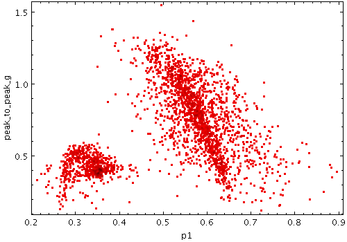
stilts plot2plane layer1=mark in1=rrlyrae.fits x1=p1 y1=peak_to_peak_g
icmdN = <cmds> (ProcessingStep[])
inN.
The value of this parameter is one or more of the filter
commands described in Section 6.1.
If more than one is given, they must be separated by
semicolon characters (";").
This parameter can be repeated multiple times on the same
command line to build up a list of processing steps.
The sequence of commands given in this way
defines the processing pipeline which is performed on the table.
Commands may alternatively be supplied in an external file,
by using the indirection character '@'.
Thus a value of "@filename"
causes the file filename to be read for a list
of filter commands to execute. The commands in the file
may be separated by newline characters and/or semicolons,
and lines which are blank or which start with a
'#' character are ignored.
A backslash character '\' at the end of a line
joins it with the following line.
ifmtN = <in-format> (String)
inN.
The known formats are listed in Section 5.1.1.
This flag can be used if you know what format your
table is in.
If it has the special value
(auto) (the default),
then an attempt will be
made to detect the format of the table automatically.
This cannot always be done correctly however, in which case
the program will exit with an error explaining which
formats were attempted.
This parameter is ignored for scheme-specified tables.
[Default: (auto)]
inN = <table> (StarTable)
-",
meaning standard input.
In this case the input format must be given explicitly
using the ifmtN
parameter.
Note that not all formats can be streamed in this way.:<scheme-name>:<scheme-args>.<" character at the start,
or a "|" character at the end
("<syscmd" or
"syscmd|").
This executes the given pipeline and reads from its
standard output.
This will probably only work on unix-like systems.istreamN = true|false (Boolean)
inN parameter
will be read as a stream.
It is necessary to give the
ifmtN parameter
in this case.
Depending on the required operations and processing mode,
this may cause the read to fail (sometimes it is necessary
to read the table more than once).
It is not normally necessary to set this flag;
in most cases the data will be streamed automatically
if that is the best thing to do.
However it can sometimes result in less resource usage when
processing large files in certain formats (such as VOTable).
This parameter is ignored for scheme-specified tables.
[Default: false]
shadingN = auto|flat|translucent|transparent|density|aux|weighted|paux|pweighted <shade-paramsN> (ShapeMode)
[Default: auto]
shapeN = filled_circle|open_circle|... (MarkerShape)
The available options are:
filled_circle
open_circle
cross
x
open_square
open_diamond
open_triangle_up
open_triangle_down
fat_circle
fat_cross
fat_x
fat_square
fat_diamond
fat_triangle_up
fat_triangle_down
filled_square
filled_diamond
filled_triangle_up
filled_triangle_down
[Default: filled_circle]
sizeN = <pixels> (Integer)
[Default: 1]
size
Plots a marker of fixed shape but variable size at each position. The size is determined by an additional input data value.
The actual size of the markers depends on the setting of the
autoscale
parameter.
If autoscaling is off, then the basic size of each marker
is the input data value in units of pixels.
If autoscaling is on, then the data values are gathered
for all the currently visible points, and a scaling factor
is applied so that the largest ones will be a sensible size
(a few tens of pixels).
This basic size can be further adjusted with the
scale factor.
Currently data values of zero always correspond to marker size of zero, negative data values are not represented, and the mapping is linear. An absolute maximum of 100 pixels is also imposed on marker sizes. Other options may be introduced in future.
Note: for marker sizes that correspond to data values in data coordinates, you may find Error plotting more appropriate.
Usage Overview:
   layerN=size shapeN=filled_circle|open_circle|... scaleN=<factor>
               autoscaleN=true|false
               shadingN=auto|flat|translucent|transparent|density|aux|weighted|paux|pweighted <shade-paramsN>
               <pos-coord-paramsN> sizeN=<num-expr> inN=<table>
               ifmtN=<in-format> istreamN=true|false icmdN=<cmds>
All the parameters listed here
affect only the relevant layer,
identified by the suffix
N.
<pos-coord-paramsN>
give a position for each row of the input table.
Their form depends on the plot geometry,
i.e. which plotting command is used.
For a plane plot (plot2plane)
the parameters would be
xN and yN.
The coordinate parameter values are in all cases strings
interpreted as numeric expressions based on column names.
These can be column names, fixed values or algebraic
expressions as described in Section 10.
Example:
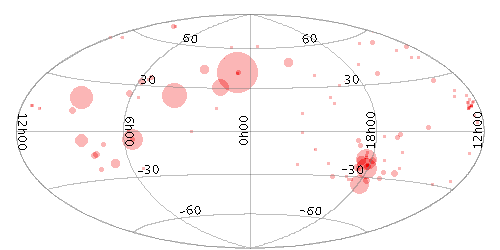
   stilts plot2sky projection=aitoff xpix=500 ypix=250
                   layer1=size in1=messier.xml shading1=transparent lon1=RA lat1=DEC size1=Radius
autoscaleN = true|false (Boolean)
If auto-scaling is off, then markers will keep exactly the same screen size during pan and zoom operations; if it's on, then the visible sizes will change according to what other points are currently plotted.
Marker size is also affected by the
scale parameter.
[Default: true]
icmdN = <cmds> (ProcessingStep[])
inN.
The value of this parameter is one or more of the filter
commands described in Section 6.1.
If more than one is given, they must be separated by
semicolon characters (";").
This parameter can be repeated multiple times on the same
command line to build up a list of processing steps.
The sequence of commands given in this way
defines the processing pipeline which is performed on the table.
Commands may alternatively be supplied in an external file,
by using the indirection character '@'.
Thus a value of "@filename"
causes the file filename to be read for a list
of filter commands to execute. The commands in the file
may be separated by newline characters and/or semicolons,
and lines which are blank or which start with a
'#' character are ignored.
A backslash character '\' at the end of a line
joins it with the following line.
ifmtN = <in-format> (String)
inN.
The known formats are listed in Section 5.1.1.
This flag can be used if you know what format your
table is in.
If it has the special value
(auto) (the default),
then an attempt will be
made to detect the format of the table automatically.
This cannot always be done correctly however, in which case
the program will exit with an error explaining which
formats were attempted.
This parameter is ignored for scheme-specified tables.
[Default: (auto)]
inN = <table> (StarTable)
-",
meaning standard input.
In this case the input format must be given explicitly
using the ifmtN
parameter.
Note that not all formats can be streamed in this way.:<scheme-name>:<scheme-args>.<" character at the start,
or a "|" character at the end
("<syscmd" or
"syscmd|").
This executes the given pipeline and reads from its
standard output.
This will probably only work on unix-like systems.istreamN = true|false (Boolean)
inN parameter
will be read as a stream.
It is necessary to give the
ifmtN parameter
in this case.
Depending on the required operations and processing mode,
this may cause the read to fail (sometimes it is necessary
to read the table more than once).
It is not normally necessary to set this flag;
in most cases the data will be streamed automatically
if that is the best thing to do.
However it can sometimes result in less resource usage when
processing large files in certain formats (such as VOTable).
This parameter is ignored for scheme-specified tables.
[Default: false]
scaleN = <factor> (Double)
[Default: 1]
shadingN = auto|flat|translucent|transparent|density|aux|weighted|paux|pweighted <shade-paramsN> (ShapeMode)
[Default: auto]
shapeN = filled_circle|open_circle|... (MarkerShape)
The available options are:
filled_circle
open_circle
cross
x
open_square
open_diamond
open_triangle_up
open_triangle_down
fat_circle
fat_cross
fat_x
fat_square
fat_diamond
fat_triangle_up
fat_triangle_down
filled_square
filled_diamond
filled_triangle_up
filled_triangle_down
[Default: filled_circle]
sizeN = <num-expr> (String)
scale
value.
The value is a numeric algebraic expression based on column names as described in Section 10.
sizexy
Plots a shaped marker with variable horizontal and vertical extents at each position. The X and Y dimensions are determined by two additional input data values.
The actual size of the markers depends on the setting of the
autoscale
parameter.
If autoscaling is off, the basic dimensions of each marker
are given by the input data values in units of pixels.
If autoscaling is on, the data values are gathered
for all the currently visible points, and scaling factors
are applied so that the largest ones will be a sensible size
(a few tens of pixels).
This autoscaling happens independently for
the X and Y directions.
The basic sizes can be further adjusted with the
scale
factor.
Currently data values of zero always correspond to marker dimension of zero, negative data values are not represented, and the mapping is linear. An absolute maximum of 100 pixels is also imposed on marker sizes. Other options may be introduced in future.
Note: for marker sizes that correspond to data values in data coordinates, you may find Error plotting more appropriate.
Usage Overview:
   layerN=sizexy shapeN=open_rectangle|open_triangle|... thickN=<int-value>
                 scaleN=<factor> autoscaleN=true|false
                 shadingN=auto|flat|translucent|transparent|density|aux|weighted|paux|pweighted <shade-paramsN>
                 <pos-coord-paramsN> xsizeN=<num-expr> ysizeN=<num-expr>
                 inN=<table> ifmtN=<in-format> istreamN=true|false icmdN=<cmds>
All the parameters listed here
affect only the relevant layer,
identified by the suffix
N.
<pos-coord-paramsN>
give a position for each row of the input table.
Their form depends on the plot geometry,
i.e. which plotting command is used.
For a plane plot (plot2plane)
the parameters would be
xN and yN.
The coordinate parameter values are in all cases strings
interpreted as numeric expressions based on column names.
These can be column names, fixed values or algebraic
expressions as described in Section 10.
Example:
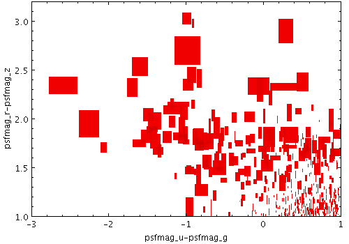
   stilts plot2plane layer1=sizexy in1=dr5qso.fits shape1=filled_rectangle
                     x1=psfmag_u-psfmag_g y1=psfmag_r-psfmag_z xsize1=exp(psfmag_g) ysize1=exp(psfmag_r)
                     xmin=-3 xmax=1 ymin=1 ymax=3.2
autoscaleN = true|false (Boolean)
If auto-scaling is off, then markers will keep exactly the same screen size during pan and zoom operations; if it's on, then the visible sizes will change according to what other points are currently plotted.
Marker size is also affected by the
scale parameter.
[Default: true]
icmdN = <cmds> (ProcessingStep[])
inN.
The value of this parameter is one or more of the filter
commands described in Section 6.1.
If more than one is given, they must be separated by
semicolon characters (";").
This parameter can be repeated multiple times on the same
command line to build up a list of processing steps.
The sequence of commands given in this way
defines the processing pipeline which is performed on the table.
Commands may alternatively be supplied in an external file,
by using the indirection character '@'.
Thus a value of "@filename"
causes the file filename to be read for a list
of filter commands to execute. The commands in the file
may be separated by newline characters and/or semicolons,
and lines which are blank or which start with a
'#' character are ignored.
A backslash character '\' at the end of a line
joins it with the following line.
ifmtN = <in-format> (String)
inN.
The known formats are listed in Section 5.1.1.
This flag can be used if you know what format your
table is in.
If it has the special value
(auto) (the default),
then an attempt will be
made to detect the format of the table automatically.
This cannot always be done correctly however, in which case
the program will exit with an error explaining which
formats were attempted.
This parameter is ignored for scheme-specified tables.
[Default: (auto)]
inN = <table> (StarTable)
-",
meaning standard input.
In this case the input format must be given explicitly
using the ifmtN
parameter.
Note that not all formats can be streamed in this way.:<scheme-name>:<scheme-args>.<" character at the start,
or a "|" character at the end
("<syscmd" or
"syscmd|").
This executes the given pipeline and reads from its
standard output.
This will probably only work on unix-like systems.istreamN = true|false (Boolean)
inN parameter
will be read as a stream.
It is necessary to give the
ifmtN parameter
in this case.
Depending on the required operations and processing mode,
this may cause the read to fail (sometimes it is necessary
to read the table more than once).
It is not normally necessary to set this flag;
in most cases the data will be streamed automatically
if that is the best thing to do.
However it can sometimes result in less resource usage when
processing large files in certain formats (such as VOTable).
This parameter is ignored for scheme-specified tables.
[Default: false]
scaleN = <factor> (Double)
[Default: 1]
shadingN = auto|flat|translucent|transparent|density|aux|weighted|paux|pweighted <shade-paramsN> (ShapeMode)
[Default: auto]
shapeN = open_rectangle|open_triangle|... (BasicXYShape)
open_rectangle
open_triangle
open_triangle_down
open_diamond
open_ellipse
filled_rectangle
filled_triangle
filled_triangle_down
filled_diamond
filled_ellipse
[Default: open_rectangle]
thickN = <int-value> (Integer)
[Default: 0]
xsizeN = <num-expr> (String)
The value is a numeric algebraic expression based on column names as described in Section 10.
ysizeN = <num-expr> (String)
The value is a numeric algebraic expression based on column names as described in Section 10.
xyvector
Plots directed lines from the data position given delta values for the coordinates. The plotted markers are typically little arrows, but there are other options.
In some cases the supplied data values
give the actual extents in data coordinates
for the plotted vectors
but sometimes the data is on a different scale
or in different units to the positional coordinates.
As a convenience for this case, the plotter can optionally
scale the magnitudes of all the vectors
to make them a reasonable size on the plot,
so by default the largest ones are a few tens of pixels long.
This auto-scaling is turned off by default,
but it can be activated with the
autoscale
option.
Whether autoscaling is on or off, the
scale
option can be used to apply a fixed scaling factor.
Usage Overview:
   layerN=xyvector arrowN=small_arrow|medium_arrow|... thickN=<int-value>
                   scaleN=<factor> autoscaleN=true|false
                   shadingN=auto|flat|translucent|transparent|density|aux|weighted|paux|pweighted <shade-paramsN>
                   xN=<num-expr> yN=<num-expr> xdeltaN=<num-expr>
                   ydeltaN=<num-expr> inN=<table> ifmtN=<in-format>
                   istreamN=true|false icmdN=<cmds>
All the parameters listed here
affect only the relevant layer,
identified by the suffix
N.
Example:
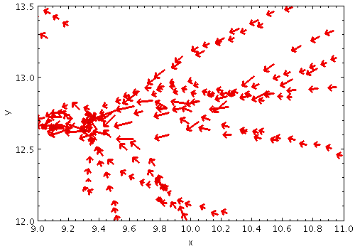
   stilts plot2plane layer1=xyvector in1=gavo_g2.fits
                     x1=x y1=y xdelta1=velX ydelta1=velY autoscale1=true thick1=1
                     xmin=9 xmax=11 ymin=12 ymax=13.5
arrowN = small_arrow|medium_arrow|... (MultiPointShape)
The available options are:
small_arrow
medium_arrow
large_arrow
small_open_dart
medium_open_dart
large_open_dart
small_filled_dart
medium_filled_dart
large_filled_dart
lines
capped_lines
[Default: small_arrow]
autoscaleN = true|false (Boolean)
If auto-scaling is on, then markers will keep approximately the same screen size during zoom operations; if it's off, they will keep the same size in data coordinates.
Marker size is also affected by the
scale parameter.
[Default: false]
icmdN = <cmds> (ProcessingStep[])
inN.
The value of this parameter is one or more of the filter
commands described in Section 6.1.
If more than one is given, they must be separated by
semicolon characters (";").
This parameter can be repeated multiple times on the same
command line to build up a list of processing steps.
The sequence of commands given in this way
defines the processing pipeline which is performed on the table.
Commands may alternatively be supplied in an external file,
by using the indirection character '@'.
Thus a value of "@filename"
causes the file filename to be read for a list
of filter commands to execute. The commands in the file
may be separated by newline characters and/or semicolons,
and lines which are blank or which start with a
'#' character are ignored.
A backslash character '\' at the end of a line
joins it with the following line.
ifmtN = <in-format> (String)
inN.
The known formats are listed in Section 5.1.1.
This flag can be used if you know what format your
table is in.
If it has the special value
(auto) (the default),
then an attempt will be
made to detect the format of the table automatically.
This cannot always be done correctly however, in which case
the program will exit with an error explaining which
formats were attempted.
This parameter is ignored for scheme-specified tables.
[Default: (auto)]
inN = <table> (StarTable)
-",
meaning standard input.
In this case the input format must be given explicitly
using the ifmtN
parameter.
Note that not all formats can be streamed in this way.:<scheme-name>:<scheme-args>.<" character at the start,
or a "|" character at the end
("<syscmd" or
"syscmd|").
This executes the given pipeline and reads from its
standard output.
This will probably only work on unix-like systems.istreamN = true|false (Boolean)
inN parameter
will be read as a stream.
It is necessary to give the
ifmtN parameter
in this case.
Depending on the required operations and processing mode,
this may cause the read to fail (sometimes it is necessary
to read the table more than once).
It is not normally necessary to set this flag;
in most cases the data will be streamed automatically
if that is the best thing to do.
However it can sometimes result in less resource usage when
processing large files in certain formats (such as VOTable).
This parameter is ignored for scheme-specified tables.
[Default: false]
scaleN = <factor> (Double)
[Default: 1]
shadingN = auto|flat|translucent|transparent|density|aux|weighted|paux|pweighted <shade-paramsN> (ShapeMode)
[Default: auto]
thickN = <int-value> (Integer)
[Default: 0]
xN = <num-expr> (String)
The value is a numeric algebraic expression based on column names as described in Section 10.
xdeltaN = <num-expr> (String)
The value is a numeric algebraic expression based on column names as described in Section 10.
yN = <num-expr> (String)
The value is a numeric algebraic expression based on column names as described in Section 10.
ydeltaN = <num-expr> (String)
The value is a numeric algebraic expression based on column names as described in Section 10.
xyerror
Plots symmetric or asymmetric error bars in some or all of the plot dimensions. The shape of the error "bars" is quite configurable, including (for 2-d and 3-d errors) ellipses, rectangles etc aligned with the axes.
Usage Overview:
   layerN=xyerror errorbarN=none|lines|capped_lines|... thickN=<int-value>
                  shadingN=auto|flat|translucent|transparent|density|aux|weighted|paux|pweighted <shade-paramsN>
                  xN=<num-expr> yN=<num-expr> xerrhiN=<num-expr>
                  xerrloN=<num-expr> yerrhiN=<num-expr> yerrloN=<num-expr>
                  inN=<table> ifmtN=<in-format> istreamN=true|false
                  icmdN=<cmds>
All the parameters listed here
affect only the relevant layer,
identified by the suffix
N.
Example:
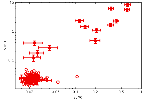
   stilts plot2plane in=J_MNRAS_440_1571.vot x=S500 y=S160
                     layer1=mark size1=5 shape1=fat_circle
                     layer2=xyerror xerrhi2=e_S500 yerrhi2=e_S160 errorbar2=capped_lines thick2=1
                     xlog=true ylog=true shading=flat xmin=0.012 xmax=1 ymin=0.01 ymax=10
errorbarN = none|lines|capped_lines|... (MultiPointShape)
The available options are:
none
lines
capped_lines
caps
arrows
ellipse
crosshair_ellipse
rectangle
crosshair_rectangle
filled_ellipse
filled_rectangle
[Default: lines]
icmdN = <cmds> (ProcessingStep[])
inN.
The value of this parameter is one or more of the filter
commands described in Section 6.1.
If more than one is given, they must be separated by
semicolon characters (";").
This parameter can be repeated multiple times on the same
command line to build up a list of processing steps.
The sequence of commands given in this way
defines the processing pipeline which is performed on the table.
Commands may alternatively be supplied in an external file,
by using the indirection character '@'.
Thus a value of "@filename"
causes the file filename to be read for a list
of filter commands to execute. The commands in the file
may be separated by newline characters and/or semicolons,
and lines which are blank or which start with a
'#' character are ignored.
A backslash character '\' at the end of a line
joins it with the following line.
ifmtN = <in-format> (String)
inN.
The known formats are listed in Section 5.1.1.
This flag can be used if you know what format your
table is in.
If it has the special value
(auto) (the default),
then an attempt will be
made to detect the format of the table automatically.
This cannot always be done correctly however, in which case
the program will exit with an error explaining which
formats were attempted.
This parameter is ignored for scheme-specified tables.
[Default: (auto)]
inN = <table> (StarTable)
-",
meaning standard input.
In this case the input format must be given explicitly
using the ifmtN
parameter.
Note that not all formats can be streamed in this way.:<scheme-name>:<scheme-args>.<" character at the start,
or a "|" character at the end
("<syscmd" or
"syscmd|").
This executes the given pipeline and reads from its
standard output.
This will probably only work on unix-like systems.istreamN = true|false (Boolean)
inN parameter
will be read as a stream.
It is necessary to give the
ifmtN parameter
in this case.
Depending on the required operations and processing mode,
this may cause the read to fail (sometimes it is necessary
to read the table more than once).
It is not normally necessary to set this flag;
in most cases the data will be streamed automatically
if that is the best thing to do.
However it can sometimes result in less resource usage when
processing large files in certain formats (such as VOTable).
This parameter is ignored for scheme-specified tables.
[Default: false]
shadingN = auto|flat|translucent|transparent|density|aux|weighted|paux|pweighted <shade-paramsN> (ShapeMode)
[Default: auto]
thickN = <int-value> (Integer)
[Default: 0]
xN = <num-expr> (String)
The value is a numeric algebraic expression based on column names as described in Section 10.
xerrhiN = <num-expr> (String)
The value is a numeric algebraic expression based on column names as described in Section 10.
xerrloN = <num-expr> (String)
The value is a numeric algebraic expression based on column names as described in Section 10.
yN = <num-expr> (String)
The value is a numeric algebraic expression based on column names as described in Section 10.
yerrhiN = <num-expr> (String)
The value is a numeric algebraic expression based on column names as described in Section 10.
yerrloN = <num-expr> (String)
The value is a numeric algebraic expression based on column names as described in Section 10.
xyellipse
Plots an ellipse (or rectangle, triangle, or other similar figure) defined by two principal radii and an optional angle of rotation, the so-called position angle. This angle, if specified, is in degrees and gives the angle counterclockwise from the horizontal axis to the first principal radius.
In some cases the supplied data values
give the actual extents in data coordinates
for the plotted ellipses
but sometimes the data is on a different scale
or in different units to the positional coordinates.
As a convenience for this case, the plotter can optionally
scale the magnitudes of all the ellipses
to make them a reasonable size on the plot,
so by default the largest ones are a few tens of pixels long.
This auto-scaling is turned off by default,
but it can be activated with the
autoscale
option.
Whether autoscaling is on or off, the
scale
option can be used to apply a fixed scaling factor.
Usage Overview:
   layerN=xyellipse ellipseN=ellipse|crosshair_ellipse|... thickN=<int-value>
                    scaleN=<factor> autoscaleN=true|false
                    shadingN=auto|flat|translucent|transparent|density|aux|weighted|paux|pweighted <shade-paramsN>
                    xN=<num-expr> yN=<num-expr> raN=<num-expr> rbN=<num-expr>
                    posangN=<deg-expr> inN=<table> ifmtN=<in-format>
                    istreamN=true|false icmdN=<cmds>
All the parameters listed here
affect only the relevant layer,
identified by the suffix
N.
Example:
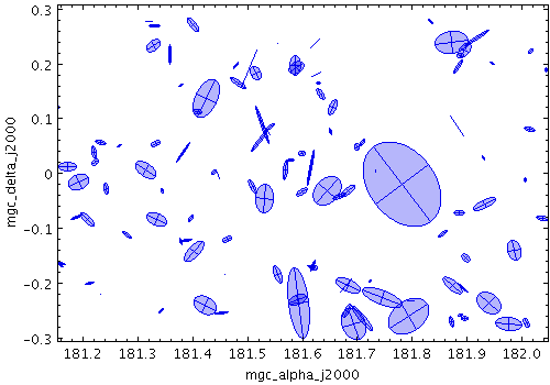
   stilts plot2plane in=mgc_ok.fits x=mgc_alpha_j2000 y=mgc_delta_j2000
                     ra=bulge_re/3600. rb=bulge_re*bulge_e/3600. posang=bulge_pa
                     autoscale=false scale=10 color=blue
                     layer1=xyellipse ellipse1=filled_ellipse shading1=transparent opaque1=4
                     layer2=xyellipse ellipse2=crosshair_ellipse
                     aspect=1 xmin=181.3 xmax=181.9
autoscaleN = true|false (Boolean)
If auto-scaling is on, then markers will keep approximately the same screen size during zoom operations; if it's off, they will keep the same size in data coordinates.
Marker size is also affected by the
scale parameter.
[Default: false]
ellipseN = ellipse|crosshair_ellipse|... (MultiPointShape)
The available options are:
ellipse
crosshair_ellipse
filled_ellipse
rectangle
crosshair_rectangle
filled_rectangle
open_triangle
filled_triangle
lines
capped_lines
arrows
[Default: ellipse]
icmdN = <cmds> (ProcessingStep[])
inN.
The value of this parameter is one or more of the filter
commands described in Section 6.1.
If more than one is given, they must be separated by
semicolon characters (";").
This parameter can be repeated multiple times on the same
command line to build up a list of processing steps.
The sequence of commands given in this way
defines the processing pipeline which is performed on the table.
Commands may alternatively be supplied in an external file,
by using the indirection character '@'.
Thus a value of "@filename"
causes the file filename to be read for a list
of filter commands to execute. The commands in the file
may be separated by newline characters and/or semicolons,
and lines which are blank or which start with a
'#' character are ignored.
A backslash character '\' at the end of a line
joins it with the following line.
ifmtN = <in-format> (String)
inN.
The known formats are listed in Section 5.1.1.
This flag can be used if you know what format your
table is in.
If it has the special value
(auto) (the default),
then an attempt will be
made to detect the format of the table automatically.
This cannot always be done correctly however, in which case
the program will exit with an error explaining which
formats were attempted.
This parameter is ignored for scheme-specified tables.
[Default: (auto)]
inN = <table> (StarTable)
-",
meaning standard input.
In this case the input format must be given explicitly
using the ifmtN
parameter.
Note that not all formats can be streamed in this way.:<scheme-name>:<scheme-args>.<" character at the start,
or a "|" character at the end
("<syscmd" or
"syscmd|").
This executes the given pipeline and reads from its
standard output.
This will probably only work on unix-like systems.istreamN = true|false (Boolean)
inN parameter
will be read as a stream.
It is necessary to give the
ifmtN parameter
in this case.
Depending on the required operations and processing mode,
this may cause the read to fail (sometimes it is necessary
to read the table more than once).
It is not normally necessary to set this flag;
in most cases the data will be streamed automatically
if that is the best thing to do.
However it can sometimes result in less resource usage when
processing large files in certain formats (such as VOTable).
This parameter is ignored for scheme-specified tables.
[Default: false]
posangN = <deg-expr> (String)
The value is a numeric algebraic expression based on column names as described in Section 10.
raN = <num-expr> (String)
The value is a numeric algebraic expression based on column names as described in Section 10.
rbN = <num-expr> (String)
The value is a numeric algebraic expression based on column names as described in Section 10.
scaleN = <factor> (Double)
[Default: 1]
shadingN = auto|flat|translucent|transparent|density|aux|weighted|paux|pweighted <shade-paramsN> (ShapeMode)
[Default: auto]
thickN = <int-value> (Integer)
[Default: 0]
xN = <num-expr> (String)
The value is a numeric algebraic expression based on column names as described in Section 10.
yN = <num-expr> (String)
The value is a numeric algebraic expression based on column names as described in Section 10.
xycorr
Plots an error ellipse (or rectangle or other similar figure) defined by errors in the X and Y directions, and a correlation between the two errors.
The supplied correlation is a dimensionless value in the range -1..+1 and is equal to the covariance divided by the product of the X and Y errors. The covariance matrix is thus:
    [  xerr*xerr         xerr*yerr*xycorr  ]
    [  xerr*yerr*xycorr  yerr*yerr         ]
In some cases the supplied data values
give the actual extents in data coordinates
for the plotted ellipses
but sometimes the data is on a different scale
or in different units to the positional coordinates.
As a convenience for this case, the plotter can optionally
scale the magnitudes of all the ellipses
to make them a reasonable size on the plot,
so by default the largest ones are a few tens of pixels long.
This auto-scaling is turned off by default,
but it can be activated with the
autoscale
option.
Whether autoscaling is on or off, the
scale
option can be used to apply a fixed scaling factor.
This plot type is suitable for use with the
<x>_error and
<x>_<y>_corr columns
in the Gaia source catalogue.
Usage Overview:
   layerN=xycorr ellipseN=ellipse|crosshair_ellipse|... thickN=<int-value>
                 scaleN=<factor> autoscaleN=true|false
                 shadingN=auto|flat|translucent|transparent|density|aux|weighted|paux|pweighted <shade-paramsN>
                 xN=<num-expr> yN=<num-expr> xerrN=<num-expr> yerrN=<num-expr>
                 xycorrN=<num-expr> inN=<table> ifmtN=<in-format>
                 istreamN=true|false icmdN=<cmds>
All the parameters listed here
affect only the relevant layer,
identified by the suffix
N.
Example:
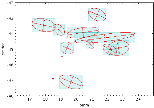
   stilts plot2plane in=tgas_source.fits icmd='select skyDistanceDegrees(ra,dec,56.9,23.9)<0.4'
                     x=pmra y=pmdec
                     layer1=mark
                     xerrhi2=pmra_error yerrhi2=pmdec_error
                     color2=cyan shading2=transparent
                     layer2a=xyerror errorbar2a=filled_rectangle opaque2a=10
                     layer2b=xyerror errorbar2b=crosshair_rectangle opaque2b=4
                     layer3=xycorr autoscale3=false
                     xerr3=pmra_error yerr3=pmdec_error xycorr3=pmra_pmdec_corr
                     ellipse3=crosshair_ellipse
                     aspect=1
                     xmin=17 xmax=24 ymin=-48 ymax=-42
autoscaleN = true|false (Boolean)
If auto-scaling is on, then markers will keep approximately the same screen size during zoom operations; if it's off, they will keep the same size in data coordinates.
Marker size is also affected by the
scale parameter.
[Default: false]
ellipseN = ellipse|crosshair_ellipse|... (MultiPointShape)
The available options are:
ellipse
crosshair_ellipse
filled_ellipse
rectangle
crosshair_rectangle
filled_rectangle
open_triangle
filled_triangle
lines
capped_lines
arrows
[Default: ellipse]
icmdN = <cmds> (ProcessingStep[])
inN.
The value of this parameter is one or more of the filter
commands described in Section 6.1.
If more than one is given, they must be separated by
semicolon characters (";").
This parameter can be repeated multiple times on the same
command line to build up a list of processing steps.
The sequence of commands given in this way
defines the processing pipeline which is performed on the table.
Commands may alternatively be supplied in an external file,
by using the indirection character '@'.
Thus a value of "@filename"
causes the file filename to be read for a list
of filter commands to execute. The commands in the file
may be separated by newline characters and/or semicolons,
and lines which are blank or which start with a
'#' character are ignored.
A backslash character '\' at the end of a line
joins it with the following line.
ifmtN = <in-format> (String)
inN.
The known formats are listed in Section 5.1.1.
This flag can be used if you know what format your
table is in.
If it has the special value
(auto) (the default),
then an attempt will be
made to detect the format of the table automatically.
This cannot always be done correctly however, in which case
the program will exit with an error explaining which
formats were attempted.
This parameter is ignored for scheme-specified tables.
[Default: (auto)]
inN = <table> (StarTable)
-",
meaning standard input.
In this case the input format must be given explicitly
using the ifmtN
parameter.
Note that not all formats can be streamed in this way.:<scheme-name>:<scheme-args>.<" character at the start,
or a "|" character at the end
("<syscmd" or
"syscmd|").
This executes the given pipeline and reads from its
standard output.
This will probably only work on unix-like systems.istreamN = true|false (Boolean)
inN parameter
will be read as a stream.
It is necessary to give the
ifmtN parameter
in this case.
Depending on the required operations and processing mode,
this may cause the read to fail (sometimes it is necessary
to read the table more than once).
It is not normally necessary to set this flag;
in most cases the data will be streamed automatically
if that is the best thing to do.
However it can sometimes result in less resource usage when
processing large files in certain formats (such as VOTable).
This parameter is ignored for scheme-specified tables.
[Default: false]
scaleN = <factor> (Double)
[Default: 1]
shadingN = auto|flat|translucent|transparent|density|aux|weighted|paux|pweighted <shade-paramsN> (ShapeMode)
[Default: auto]
thickN = <int-value> (Integer)
[Default: 0]
xN = <num-expr> (String)
The value is a numeric algebraic expression based on column names as described in Section 10.
xerrN = <num-expr> (String)
The value is a numeric algebraic expression based on column names as described in Section 10.
xycorrN = <num-expr> (String)
*_corr values
supplied in the Gaia source catalogue.
The value is a numeric algebraic expression based on column names as described in Section 10.
yN = <num-expr> (String)
The value is a numeric algebraic expression based on column names as described in Section 10.
yerrN = <num-expr> (String)
The value is a numeric algebraic expression based on column names as described in Section 10.
link2
Plots a line linking two positions from the same input table row.
Usage Overview:
   layerN=link2 thickN=<int-value>
                shadingN=auto|flat|translucent|transparent|density|aux|weighted|paux|pweighted <shade-paramsN>
                <pos-coord-params1N> <pos-coord-params2N> inN=<table>
                ifmtN=<in-format> istreamN=true|false icmdN=<cmds>
All the parameters listed here
affect only the relevant layer,
identified by the suffix
N.
<pos-coord-params1N>
, <pos-coord-params2N>
give 2 positions for each row of the input table.
Their form depends on the plot geometry,
i.e. which plotting command is used.
For a plane plot (plot2plane)
the parameters would be
x1N, y1N,
x2N and y2N.
The coordinate parameter values are in all cases strings
interpreted as numeric expressions based on column names.
These can be column names, fixed values or algebraic
expressions as described in Section 10.
Example:
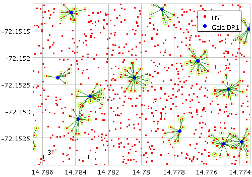
   stilts plot2sky clon=14.78 clat=-72.1525 radius=0.0015 sex=false
                   layer_h=mark in_h=ngc346.fits lon_h=_RAJ2000 lat_h=_DEJ2000 color_h=red
                   layer_g=mark in_g=ngc346xGaiadr1.fits lon_g=ra lat_g=dec color_g=blue shading_g=flat size_g=3
                   in_x=ngc346xGaiadr1.fits lon1_x=_RAJ2000 lat1_x=_DEJ2000 lon2_x=ra lat2_x=dec shading_x=flat
                   layer_xl=link2 color_xl=forestgreen
                   layer_xm=mark2 color_xm=greenyellow size_xm=4 shape_xm=open_circle
                   seq=_xm,_xl,_h,_g leglabel_h=HST leglabel_g='Gaia DR1' legseq=_h,_g legpos=0.95,0.95
icmdN = <cmds> (ProcessingStep[])
inN.
The value of this parameter is one or more of the filter
commands described in Section 6.1.
If more than one is given, they must be separated by
semicolon characters (";").
This parameter can be repeated multiple times on the same
command line to build up a list of processing steps.
The sequence of commands given in this way
defines the processing pipeline which is performed on the table.
Commands may alternatively be supplied in an external file,
by using the indirection character '@'.
Thus a value of "@filename"
causes the file filename to be read for a list
of filter commands to execute. The commands in the file
may be separated by newline characters and/or semicolons,
and lines which are blank or which start with a
'#' character are ignored.
A backslash character '\' at the end of a line
joins it with the following line.
ifmtN = <in-format> (String)
inN.
The known formats are listed in Section 5.1.1.
This flag can be used if you know what format your
table is in.
If it has the special value
(auto) (the default),
then an attempt will be
made to detect the format of the table automatically.
This cannot always be done correctly however, in which case
the program will exit with an error explaining which
formats were attempted.
This parameter is ignored for scheme-specified tables.
[Default: (auto)]
inN = <table> (StarTable)
-",
meaning standard input.
In this case the input format must be given explicitly
using the ifmtN
parameter.
Note that not all formats can be streamed in this way.:<scheme-name>:<scheme-args>.<" character at the start,
or a "|" character at the end
("<syscmd" or
"syscmd|").
This executes the given pipeline and reads from its
standard output.
This will probably only work on unix-like systems.istreamN = true|false (Boolean)
inN parameter
will be read as a stream.
It is necessary to give the
ifmtN parameter
in this case.
Depending on the required operations and processing mode,
this may cause the read to fail (sometimes it is necessary
to read the table more than once).
It is not normally necessary to set this flag;
in most cases the data will be streamed automatically
if that is the best thing to do.
However it can sometimes result in less resource usage when
processing large files in certain formats (such as VOTable).
This parameter is ignored for scheme-specified tables.
[Default: false]
shadingN = auto|flat|translucent|transparent|density|aux|weighted|paux|pweighted <shade-paramsN> (ShapeMode)
[Default: auto]
thickN = <int-value> (Integer)
[Default: 0]
mark2
Plots 2 similar markers of fixed size and shape representing 2 separate positions from the same input table row. This is a convenience option that can be used with other plot layers based on 2 positions.
Usage Overview:
   layerN=mark2 shapeN=filled_circle|open_circle|... sizeN=<pixels>
                shadingN=auto|flat|translucent|transparent|density|aux|weighted|paux|pweighted <shade-paramsN>
                <pos-coord-params1N> <pos-coord-params2N> inN=<table>
                ifmtN=<in-format> istreamN=true|false icmdN=<cmds>
All the parameters listed here
affect only the relevant layer,
identified by the suffix
N.
<pos-coord-params1N>
, <pos-coord-params2N>
give 2 positions for each row of the input table.
Their form depends on the plot geometry,
i.e. which plotting command is used.
For a plane plot (plot2plane)
the parameters would be
x1N, y1N,
x2N and y2N.
The coordinate parameter values are in all cases strings
interpreted as numeric expressions based on column names.
These can be column names, fixed values or algebraic
expressions as described in Section 10.
Example:
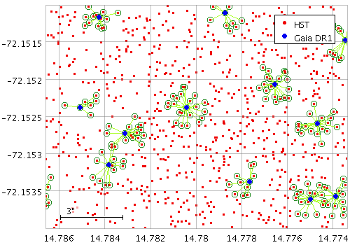
   stilts plot2sky clon=14.78 clat=-72.1525 radius=0.0015 sex=false
                   layer_h=mark in_h=ngc346.fits lon_h=_RAJ2000 lat_h=_DEJ2000 color_h=red
                   layer_g=mark in_g=ngc346xGaiadr1.fits lon_g=ra lat_g=dec color_g=blue shading_g=flat size_g=3
                   in_x=ngc346xGaiadr1.fits lon1_x=_RAJ2000 lat1_x=_DEJ2000 lon2_x=ra lat2_x=dec shading_x=flat
                   layer_xl=link2 color_xl=greenyellow
                   layer_xm=mark2 color_xm=forestgreen size_xm=4 shape_xm=open_circle
                   seq=_xm,_xl,_h,_g leglabel_h=HST leglabel_g='Gaia DR1' legseq=_h,_g legpos=0.95,0.95
icmdN = <cmds> (ProcessingStep[])
inN.
The value of this parameter is one or more of the filter
commands described in Section 6.1.
If more than one is given, they must be separated by
semicolon characters (";").
This parameter can be repeated multiple times on the same
command line to build up a list of processing steps.
The sequence of commands given in this way
defines the processing pipeline which is performed on the table.
Commands may alternatively be supplied in an external file,
by using the indirection character '@'.
Thus a value of "@filename"
causes the file filename to be read for a list
of filter commands to execute. The commands in the file
may be separated by newline characters and/or semicolons,
and lines which are blank or which start with a
'#' character are ignored.
A backslash character '\' at the end of a line
joins it with the following line.
ifmtN = <in-format> (String)
inN.
The known formats are listed in Section 5.1.1.
This flag can be used if you know what format your
table is in.
If it has the special value
(auto) (the default),
then an attempt will be
made to detect the format of the table automatically.
This cannot always be done correctly however, in which case
the program will exit with an error explaining which
formats were attempted.
This parameter is ignored for scheme-specified tables.
[Default: (auto)]
inN = <table> (StarTable)
-",
meaning standard input.
In this case the input format must be given explicitly
using the ifmtN
parameter.
Note that not all formats can be streamed in this way.:<scheme-name>:<scheme-args>.<" character at the start,
or a "|" character at the end
("<syscmd" or
"syscmd|").
This executes the given pipeline and reads from its
standard output.
This will probably only work on unix-like systems.istreamN = true|false (Boolean)
inN parameter
will be read as a stream.
It is necessary to give the
ifmtN parameter
in this case.
Depending on the required operations and processing mode,
this may cause the read to fail (sometimes it is necessary
to read the table more than once).
It is not normally necessary to set this flag;
in most cases the data will be streamed automatically
if that is the best thing to do.
However it can sometimes result in less resource usage when
processing large files in certain formats (such as VOTable).
This parameter is ignored for scheme-specified tables.
[Default: false]
shadingN = auto|flat|translucent|transparent|density|aux|weighted|paux|pweighted <shade-paramsN> (ShapeMode)
[Default: auto]
shapeN = filled_circle|open_circle|... (MarkerShape)
The available options are:
filled_circle
open_circle
cross
x
open_square
open_diamond
open_triangle_up
open_triangle_down
fat_circle
fat_cross
fat_x
fat_square
fat_diamond
fat_triangle_up
fat_triangle_down
filled_square
filled_diamond
filled_triangle_up
filled_triangle_down
[Default: filled_circle]
sizeN = <pixels> (Integer)
[Default: 1]
poly4
Draws a closed quadrilateral
given the coordinates of its vertices
supplied as 4 separate positions.
The way that the polygon is drawn (outline, fill etc)
is determined using the
polymode
option.
Polygons smaller than a configurable threshold size in pixels are by default represented by a replacement marker, so the position of even a very small polygon is still visible on the screen.
Usage Overview:
   layerN=poly4 polymodeN=outline|border|fill|cross|star thickN=<int-value>
                minsizeN=<pixels> minshapeN=filled_circle|open_circle|...
                shadingN=auto|flat|translucent|transparent|density|aux|weighted|paux|pweighted <shade-paramsN>
                <pos-coord-params1N> <pos-coord-params2N> <pos-coord-params3N>
                <pos-coord-params4N> inN=<table> ifmtN=<in-format>
                istreamN=true|false icmdN=<cmds>
All the parameters listed here
affect only the relevant layer,
identified by the suffix
N.
<pos-coord-params1N>
, <pos-coord-params2N>
, <pos-coord-params3N>
, <pos-coord-params4N>
give 4 positions for each row of the input table.
Their form depends on the plot geometry,
i.e. which plotting command is used.
For a plane plot (plot2plane)
the parameters would be
x1N, y1N,
x2N, y2N,
x3N, y3N,
x4N and y4N.
The coordinate parameter values are in all cases strings
interpreted as numeric expressions based on column names.
These can be column names, fixed values or algebraic
expressions as described in Section 10.
Example:
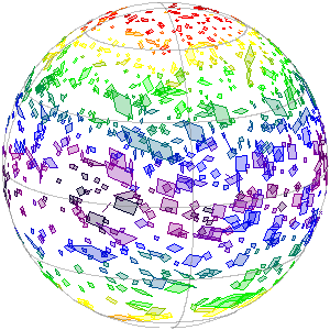
   stilts plot2sky in=big_tab_VIR_VIS_CSA_public.fits icmd='every 32'
                   lon1=LON_CORNER_1 lat1=LAT_CORNER_1
                   lon2=LON_CORNER_2 lat2=LAT_CORNER_2
                   lon3=LON_CORNER_3 lat3=LAT_CORNER_3
                   lon4=LON_CORNER_4 lat4=LAT_CORNER_4
                   aux=RADIUS
                   layer_o=poly4 polymode_o=outline shading_o=aux
                   layer_f=poly4 polymode_f=fill shading_f=aux opaque_f=4
                   auxmap=rainbow auxvisible=false xpix=300 ypix=300 labelpos=none
icmdN = <cmds> (ProcessingStep[])
inN.
The value of this parameter is one or more of the filter
commands described in Section 6.1.
If more than one is given, they must be separated by
semicolon characters (";").
This parameter can be repeated multiple times on the same
command line to build up a list of processing steps.
The sequence of commands given in this way
defines the processing pipeline which is performed on the table.
Commands may alternatively be supplied in an external file,
by using the indirection character '@'.
Thus a value of "@filename"
causes the file filename to be read for a list
of filter commands to execute. The commands in the file
may be separated by newline characters and/or semicolons,
and lines which are blank or which start with a
'#' character are ignored.
A backslash character '\' at the end of a line
joins it with the following line.
ifmtN = <in-format> (String)
inN.
The known formats are listed in Section 5.1.1.
This flag can be used if you know what format your
table is in.
If it has the special value
(auto) (the default),
then an attempt will be
made to detect the format of the table automatically.
This cannot always be done correctly however, in which case
the program will exit with an error explaining which
formats were attempted.
This parameter is ignored for scheme-specified tables.
[Default: (auto)]
inN = <table> (StarTable)
-",
meaning standard input.
In this case the input format must be given explicitly
using the ifmtN
parameter.
Note that not all formats can be streamed in this way.:<scheme-name>:<scheme-args>.<" character at the start,
or a "|" character at the end
("<syscmd" or
"syscmd|").
This executes the given pipeline and reads from its
standard output.
This will probably only work on unix-like systems.istreamN = true|false (Boolean)
inN parameter
will be read as a stream.
It is necessary to give the
ifmtN parameter
in this case.
Depending on the required operations and processing mode,
this may cause the read to fail (sometimes it is necessary
to read the table more than once).
It is not normally necessary to set this flag;
in most cases the data will be streamed automatically
if that is the best thing to do.
However it can sometimes result in less resource usage when
processing large files in certain formats (such as VOTable).
This parameter is ignored for scheme-specified tables.
[Default: false]
minshapeN = filled_circle|open_circle|... (MarkerShape)
minsize.
The available options are:
filled_circle
open_circle
cross
x
open_square
open_diamond
open_triangle_up
open_triangle_down
fat_circle
fat_cross
fat_x
fat_square
fat_diamond
fat_triangle_up
fat_triangle_down
filled_square
filled_diamond
filled_triangle_up
filled_triangle_down
[Default: x]
minsizeN = <pixels> (Integer)
[Default: 1]
polymodeN = outline|border|fill|cross|star (PolygonShape)
The available options are:
outline: draws a line round the outside of the polygonborder: draws a line butting up to the outside of the polygon; may look better for adjacent shapes, but more expensive to drawfill: fills the interior of the polygoncross: draws a line round the outside of the polygon and lines between all the verticesstar: draws a line round the outside of the polygon and lines from the nominal center to each vertex[Default: outline]
shadingN = auto|flat|translucent|transparent|density|aux|weighted|paux|pweighted <shade-paramsN> (ShapeMode)
[Default: auto]
thickN = <int-value> (Integer)
[Default: 0]
mark4
Plots 4 similar markers of fixed size and shape representing 4 separate positions from the same input table row. This is a convenience option that can be used with other plot layers based on 4 positions.
Usage Overview:
   layerN=mark4 shapeN=filled_circle|open_circle|... sizeN=<pixels>
                shadingN=auto|flat|translucent|transparent|density|aux|weighted|paux|pweighted <shade-paramsN>
                <pos-coord-params1N> <pos-coord-params2N> <pos-coord-params3N>
                <pos-coord-params4N> inN=<table> ifmtN=<in-format>
                istreamN=true|false icmdN=<cmds>
All the parameters listed here
affect only the relevant layer,
identified by the suffix
N.
<pos-coord-params1N>
, <pos-coord-params2N>
, <pos-coord-params3N>
, <pos-coord-params4N>
give 4 positions for each row of the input table.
Their form depends on the plot geometry,
i.e. which plotting command is used.
For a plane plot (plot2plane)
the parameters would be
x1N, y1N,
x2N, y2N,
x3N, y3N,
x4N and y4N.
The coordinate parameter values are in all cases strings
interpreted as numeric expressions based on column names.
These can be column names, fixed values or algebraic
expressions as described in Section 10.
Example:
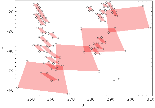
   stilts plot2plane in=big_tab_VIR_VIS_CSA_public.fits
                     icmd='select IOF_055<0.005'
                     icmd='select lon_center>250&&lon_center<300&&lat_center>-65&&lat_center<-16'
                     x1=LON_CORNER_1 y1=LAT_CORNER_1
                     x2=LON_CORNER_2 y2=LAT_CORNER_2
                     x3=LON_CORNER_3 y3=LAT_CORNER_3
                     x4=LON_CORNER_4 y4=LAT_CORNER_4
                     layer_q=poly4 polymode_q=fill shading_q=transparent opaque_q=4
                     layer_m=mark4 color_m=404040 shape_m=open_circle size_m=3
icmdN = <cmds> (ProcessingStep[])
inN.
The value of this parameter is one or more of the filter
commands described in Section 6.1.
If more than one is given, they must be separated by
semicolon characters (";").
This parameter can be repeated multiple times on the same
command line to build up a list of processing steps.
The sequence of commands given in this way
defines the processing pipeline which is performed on the table.
Commands may alternatively be supplied in an external file,
by using the indirection character '@'.
Thus a value of "@filename"
causes the file filename to be read for a list
of filter commands to execute. The commands in the file
may be separated by newline characters and/or semicolons,
and lines which are blank or which start with a
'#' character are ignored.
A backslash character '\' at the end of a line
joins it with the following line.
ifmtN = <in-format> (String)
inN.
The known formats are listed in Section 5.1.1.
This flag can be used if you know what format your
table is in.
If it has the special value
(auto) (the default),
then an attempt will be
made to detect the format of the table automatically.
This cannot always be done correctly however, in which case
the program will exit with an error explaining which
formats were attempted.
This parameter is ignored for scheme-specified tables.
[Default: (auto)]
inN = <table> (StarTable)
-",
meaning standard input.
In this case the input format must be given explicitly
using the ifmtN
parameter.
Note that not all formats can be streamed in this way.:<scheme-name>:<scheme-args>.<" character at the start,
or a "|" character at the end
("<syscmd" or
"syscmd|").
This executes the given pipeline and reads from its
standard output.
This will probably only work on unix-like systems.istreamN = true|false (Boolean)
inN parameter
will be read as a stream.
It is necessary to give the
ifmtN parameter
in this case.
Depending on the required operations and processing mode,
this may cause the read to fail (sometimes it is necessary
to read the table more than once).
It is not normally necessary to set this flag;
in most cases the data will be streamed automatically
if that is the best thing to do.
However it can sometimes result in less resource usage when
processing large files in certain formats (such as VOTable).
This parameter is ignored for scheme-specified tables.
[Default: false]
shadingN = auto|flat|translucent|transparent|density|aux|weighted|paux|pweighted <shade-paramsN> (ShapeMode)
[Default: auto]
shapeN = filled_circle|open_circle|... (MarkerShape)
The available options are:
filled_circle
open_circle
cross
x
open_square
open_diamond
open_triangle_up
open_triangle_down
fat_circle
fat_cross
fat_x
fat_square
fat_diamond
fat_triangle_up
fat_triangle_down
filled_square
filled_diamond
filled_triangle_up
filled_triangle_down
[Default: filled_circle]
sizeN = <pixels> (Integer)
[Default: 1]
polygon
Draws a closed polygon given an array of coordinates
that define its vertices.
In fact this plot requires the position of the first vertex
supplied as a positional value in the usual way
(e.g. X and Y coordinates)
and the second, third etc vertices supplied as an array
using the otherpoints parameter.
Invocation might therefore look like
"xN=x1 yN=y1 otherpointsN=array(x2,y2, x3,y3, x4,y4)".
Usage Overview:
   layerN=polygon useposN=true|false polymodeN=outline|border|fill|cross|star
                  thickN=<int-value>
                  shadingN=auto|flat|translucent|transparent|density|aux|weighted|paux|pweighted <shade-paramsN>
                  <pos-coord-paramsN> otherpointsN=<array-expr> inN=<table>
                  ifmtN=<in-format> istreamN=true|false icmdN=<cmds>
All the parameters listed here
affect only the relevant layer,
identified by the suffix
N.
<pos-coord-paramsN>
give a position for each row of the input table.
Their form depends on the plot geometry,
i.e. which plotting command is used.
For a plane plot (plot2plane)
the parameters would be
xN and yN.
The coordinate parameter values are in all cases strings
interpreted as numeric expressions based on column names.
These can be column names, fixed values or algebraic
expressions as described in Section 10.
Example:
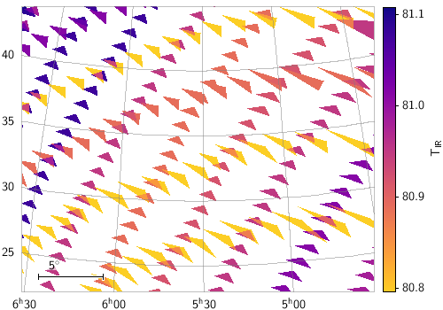
   stilts plot2sky in=big_tab_VIR_VIS_CSA_public.fits
                   icmd='select ALTITUDE>4e4&&ALTITUDE<4.3e4'
                   layer=polygon polymode=fill
                   lon=LON_CENTER lat=LAT_CENTER
                   otherpoints=array(lon_corner_1,lat_corner_1,lon_corner_2,lat_corner_2)
                   shading=weighted weight=IR_TEMPERATURE auxmap=plasma
                   texttype=latex fontsize=14 auxlabel=T_{IR}
                   clon=83 clat=34 radius=11
icmdN = <cmds> (ProcessingStep[])
inN.
The value of this parameter is one or more of the filter
commands described in Section 6.1.
If more than one is given, they must be separated by
semicolon characters (";").
This parameter can be repeated multiple times on the same
command line to build up a list of processing steps.
The sequence of commands given in this way
defines the processing pipeline which is performed on the table.
Commands may alternatively be supplied in an external file,
by using the indirection character '@'.
Thus a value of "@filename"
causes the file filename to be read for a list
of filter commands to execute. The commands in the file
may be separated by newline characters and/or semicolons,
and lines which are blank or which start with a
'#' character are ignored.
A backslash character '\' at the end of a line
joins it with the following line.
ifmtN = <in-format> (String)
inN.
The known formats are listed in Section 5.1.1.
This flag can be used if you know what format your
table is in.
If it has the special value
(auto) (the default),
then an attempt will be
made to detect the format of the table automatically.
This cannot always be done correctly however, in which case
the program will exit with an error explaining which
formats were attempted.
This parameter is ignored for scheme-specified tables.
[Default: (auto)]
inN = <table> (StarTable)
-",
meaning standard input.
In this case the input format must be given explicitly
using the ifmtN
parameter.
Note that not all formats can be streamed in this way.:<scheme-name>:<scheme-args>.<" character at the start,
or a "|" character at the end
("<syscmd" or
"syscmd|").
This executes the given pipeline and reads from its
standard output.
This will probably only work on unix-like systems.istreamN = true|false (Boolean)
inN parameter
will be read as a stream.
It is necessary to give the
ifmtN parameter
in this case.
Depending on the required operations and processing mode,
this may cause the read to fail (sometimes it is necessary
to read the table more than once).
It is not normally necessary to set this flag;
in most cases the data will be streamed automatically
if that is the best thing to do.
However it can sometimes result in less resource usage when
processing large files in certain formats (such as VOTable).
This parameter is ignored for scheme-specified tables.
[Default: false]
otherpointsN = <array-expr> (String)
usepos
parameter.
Some expression language functions that can be useful
when specifying this parameter are
array() and parseDoubles().
The value is an array-valued algebraic expression based on column names as described in Section 10. Some of the functions in the Arrays class may be useful here.
polymodeN = outline|border|fill|cross|star (PolygonShape)
The available options are:
outline: draws a line round the outside of the polygonborder: draws a line butting up to the outside of the polygon; may look better for adjacent shapes, but more expensive to drawfill: fills the interior of the polygoncross: draws a line round the outside of the polygon and lines between all the verticesstar: draws a line round the outside of the polygon and lines from the nominal center to each vertex[Default: outline]
shadingN = auto|flat|translucent|transparent|density|aux|weighted|paux|pweighted <shade-paramsN> (ShapeMode)
[Default: auto]
thickN = <int-value> (Integer)
[Default: 0]
useposN = true|false (Boolean)
[Default: true]
area
Plots a region on the plotting surface
specified by a string or array of numbers.
The area may be specified as an STC-S string
(as for example in an ObsCore or EPN-TAP
s_region column)
or using an array of numbers representing a
polygon, circle or point as flagged using the DALI/VOTable
extended type (xtype) marker,
or as an ASCII-encoded MOC.
Areas smaller than a configurable threshold size in pixels are by default represented by a replacement marker, so the position of even a very small area is still visible on the screen.
This plot type is generally intended for displaying relatively small shapes such as instrument footprints. It can be used for areas that are larger as well, but there may be issues with use, for instance auto-determination of the initial plot region may not work so well, and the rendering of shapes that are large relative to the sky may be inaccurate. These issues may be addressed in future releases.
Usage Overview:
   layerN=area polymodeN=outline|border|fill|cross|star thickN=<int-value>
               minsizeN=<pixels> minshapeN=filled_circle|open_circle|...
               shadingN=auto|flat|translucent|transparent|density|aux|weighted|paux|pweighted <shade-paramsN>
               areaN=<area-expr>
               areatypeN=POINT|CIRCLE|POLYGON|MOC-ASCII|UNIQ|STC-S|TFCAT
               inN=<table> ifmtN=<in-format> istreamN=true|false icmdN=<cmds>
All the parameters listed here
affect only the relevant layer,
identified by the suffix
N.
Example:
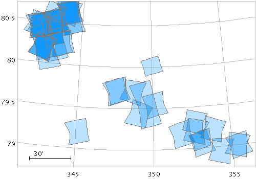
   stilts plot2sky reflectlon=false sex=false clon=348.9 clat=79.8 radius=1.0
                   in=crism.fits icmd='select sensor_id==0x4c'
                   area_p=s_region areatype_p=stc-s
                   layer_pf=area polymode_pf=fill color_pf=1199ff shading_pf=transparent
                   layer_pl=area polymode_pl=outline color_pl=grey
areaN = <area-expr> (String)
areatype parameter.
The value is a Area value algebraic expression based on column names as described in Section 10.
areatypeN = POINT|CIRCLE|POLYGON|MOC-ASCII|UNIQ|STC-S|TFCAT (AreaMapper)
areaN is supplied.
Options are:
POINT: 2-element array (x,y)CIRCLE: 3-element array (x, y, r)POLYGON: 2n-element array (x1,y1, x2,y2,...);
a NaN,NaN pair can be used to delimit distinct polygons.MOC-ASCII: Region description using ASCII MOC syntax;
see MOC 2.0 sec 4.3.2.
Note there are currently a few issues
with MOC plotting, especially for large pixels.UNIQ: Region description representing a single HEALPix cell
as defined by an UNIQ value, see
MOC 2.0
sec 4.3.1.STC-S: Region description using STC-S syntax;
see TAP 1.0, section 6.
Note there are some restrictions:
<frame>, <refpos> and <flavor> metadata are ignored,
polygon winding direction is ignored (small polygons are assumed)
and the INTERSECTION and NOT constructions are not supported.
The non-standard MOC construction is supported.TFCAT: Time-Frequency region defined by the
TFCat standard.
Support is currently incomplete;
holes in Polygons and MultiPolygons are not displayed correctly,
single Points may not be displayed,
and Coordinate Reference System information is ignored.
areaN value.
icmdN = <cmds> (ProcessingStep[])
inN.
The value of this parameter is one or more of the filter
commands described in Section 6.1.
If more than one is given, they must be separated by
semicolon characters (";").
This parameter can be repeated multiple times on the same
command line to build up a list of processing steps.
The sequence of commands given in this way
defines the processing pipeline which is performed on the table.
Commands may alternatively be supplied in an external file,
by using the indirection character '@'.
Thus a value of "@filename"
causes the file filename to be read for a list
of filter commands to execute. The commands in the file
may be separated by newline characters and/or semicolons,
and lines which are blank or which start with a
'#' character are ignored.
A backslash character '\' at the end of a line
joins it with the following line.
ifmtN = <in-format> (String)
inN.
The known formats are listed in Section 5.1.1.
This flag can be used if you know what format your
table is in.
If it has the special value
(auto) (the default),
then an attempt will be
made to detect the format of the table automatically.
This cannot always be done correctly however, in which case
the program will exit with an error explaining which
formats were attempted.
This parameter is ignored for scheme-specified tables.
[Default: (auto)]
inN = <table> (StarTable)
-",
meaning standard input.
In this case the input format must be given explicitly
using the ifmtN
parameter.
Note that not all formats can be streamed in this way.:<scheme-name>:<scheme-args>.<" character at the start,
or a "|" character at the end
("<syscmd" or
"syscmd|").
This executes the given pipeline and reads from its
standard output.
This will probably only work on unix-like systems.istreamN = true|false (Boolean)
inN parameter
will be read as a stream.
It is necessary to give the
ifmtN parameter
in this case.
Depending on the required operations and processing mode,
this may cause the read to fail (sometimes it is necessary
to read the table more than once).
It is not normally necessary to set this flag;
in most cases the data will be streamed automatically
if that is the best thing to do.
However it can sometimes result in less resource usage when
processing large files in certain formats (such as VOTable).
This parameter is ignored for scheme-specified tables.
[Default: false]
minshapeN = filled_circle|open_circle|... (MarkerShape)
minsize.
The available options are:
filled_circle
open_circle
cross
x
open_square
open_diamond
open_triangle_up
open_triangle_down
fat_circle
fat_cross
fat_x
fat_square
fat_diamond
fat_triangle_up
fat_triangle_down
filled_square
filled_diamond
filled_triangle_up
filled_triangle_down
[Default: x]
minsizeN = <pixels> (Integer)
[Default: 1]
polymodeN = outline|border|fill|cross|star (PolygonShape)
The available options are:
outline: draws a line round the outside of the polygonborder: draws a line butting up to the outside of the polygon; may look better for adjacent shapes, but more expensive to drawfill: fills the interior of the polygoncross: draws a line round the outside of the polygon and lines between all the verticesstar: draws a line round the outside of the polygon and lines from the nominal center to each vertex[Default: outline]
shadingN = auto|flat|translucent|transparent|density|aux|weighted|paux|pweighted <shade-paramsN> (ShapeMode)
[Default: auto]
thickN = <int-value> (Integer)
[Default: 0]
central
Plots the nominal central point of an area. This appears just like a normal marker plot, but can be used when the available geometry information is an area description (such as an STC-S string or an array of polygon vertices) rather than coordinate values such as an X,Y pair. The position plotted is the nominal center of the shape as determined by the plotting code; that may or may not correspond to the actual center.
Usage Overview:
   layerN=central shapeN=filled_circle|open_circle|... sizeN=<pixels>
                  shadingN=auto|flat|translucent|transparent|density|aux|weighted|paux|pweighted <shade-paramsN>
                  areaN=<area-expr>
                  areatypeN=POINT|CIRCLE|POLYGON|MOC-ASCII|UNIQ|STC-S|TFCAT
                  inN=<table> ifmtN=<in-format> istreamN=true|false
                  icmdN=<cmds>
All the parameters listed here
affect only the relevant layer,
identified by the suffix
N.
Example:
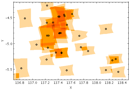
   stilts plot2plane xmin=136.7 xmax=138.5 ymin=-5.7 ymax=-4.2
                     in=crism.fits icmd='select sensor_id==0x53'
                     area=s_region areatype=STC-S
                     layer1=area polymode1=fill shading1=density densemap1=heat
                     layer2=central shape2=fat_circle size2=3 color2=black
areaN = <area-expr> (String)
areatype parameter.
The value is a Area value algebraic expression based on column names as described in Section 10.
areatypeN = POINT|CIRCLE|POLYGON|MOC-ASCII|UNIQ|STC-S|TFCAT (AreaMapper)
areaN is supplied.
Options are:
POINT: 2-element array (x,y)CIRCLE: 3-element array (x, y, r)POLYGON: 2n-element array (x1,y1, x2,y2,...);
a NaN,NaN pair can be used to delimit distinct polygons.MOC-ASCII: Region description using ASCII MOC syntax;
see MOC 2.0 sec 4.3.2.
Note there are currently a few issues
with MOC plotting, especially for large pixels.UNIQ: Region description representing a single HEALPix cell
as defined by an UNIQ value, see
MOC 2.0
sec 4.3.1.STC-S: Region description using STC-S syntax;
see TAP 1.0, section 6.
Note there are some restrictions:
<frame>, <refpos> and <flavor> metadata are ignored,
polygon winding direction is ignored (small polygons are assumed)
and the INTERSECTION and NOT constructions are not supported.
The non-standard MOC construction is supported.TFCAT: Time-Frequency region defined by the
TFCat standard.
Support is currently incomplete;
holes in Polygons and MultiPolygons are not displayed correctly,
single Points may not be displayed,
and Coordinate Reference System information is ignored.
areaN value.
icmdN = <cmds> (ProcessingStep[])
inN.
The value of this parameter is one or more of the filter
commands described in Section 6.1.
If more than one is given, they must be separated by
semicolon characters (";").
This parameter can be repeated multiple times on the same
command line to build up a list of processing steps.
The sequence of commands given in this way
defines the processing pipeline which is performed on the table.
Commands may alternatively be supplied in an external file,
by using the indirection character '@'.
Thus a value of "@filename"
causes the file filename to be read for a list
of filter commands to execute. The commands in the file
may be separated by newline characters and/or semicolons,
and lines which are blank or which start with a
'#' character are ignored.
A backslash character '\' at the end of a line
joins it with the following line.
ifmtN = <in-format> (String)
inN.
The known formats are listed in Section 5.1.1.
This flag can be used if you know what format your
table is in.
If it has the special value
(auto) (the default),
then an attempt will be
made to detect the format of the table automatically.
This cannot always be done correctly however, in which case
the program will exit with an error explaining which
formats were attempted.
This parameter is ignored for scheme-specified tables.
[Default: (auto)]
inN = <table> (StarTable)
-",
meaning standard input.
In this case the input format must be given explicitly
using the ifmtN
parameter.
Note that not all formats can be streamed in this way.:<scheme-name>:<scheme-args>.<" character at the start,
or a "|" character at the end
("<syscmd" or
"syscmd|").
This executes the given pipeline and reads from its
standard output.
This will probably only work on unix-like systems.istreamN = true|false (Boolean)
inN parameter
will be read as a stream.
It is necessary to give the
ifmtN parameter
in this case.
Depending on the required operations and processing mode,
this may cause the read to fail (sometimes it is necessary
to read the table more than once).
It is not normally necessary to set this flag;
in most cases the data will be streamed automatically
if that is the best thing to do.
However it can sometimes result in less resource usage when
processing large files in certain formats (such as VOTable).
This parameter is ignored for scheme-specified tables.
[Default: false]
shadingN = auto|flat|translucent|transparent|density|aux|weighted|paux|pweighted <shade-paramsN> (ShapeMode)
[Default: auto]
shapeN = filled_circle|open_circle|... (MarkerShape)
The available options are:
filled_circle
open_circle
cross
x
open_square
open_diamond
open_triangle_up
open_triangle_down
fat_circle
fat_cross
fat_x
fat_square
fat_diamond
fat_triangle_up
fat_triangle_down
filled_square
filled_diamond
filled_triangle_up
filled_triangle_down
[Default: filled_circle]
sizeN = <pixels> (Integer)
[Default: 1]
lines
Plots an N-segment line for each input row, with the X and Y coordinate arrays each supplied by an N-element array value.
Usage Overview:
   layerN=lines thickN=<pixels> dashN=dot|dash|...|<a,b,...> sortaxisN=[X|Y]
                shadingN=auto|flat|translucent|transparent|density|aux|weighted|paux|pweighted <shade-paramsN>
                xsN=<array-expr> ysN=<array-expr> inN=<table> ifmtN=<in-format>
                istreamN=true|false icmdN=<cmds>
All the parameters listed here
affect only the relevant layer,
identified by the suffix
N.
Example:
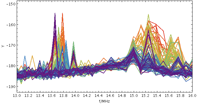
   stilts plot2plane in1=LRS_NPW_V010_20071101.cdf
                     layer1=lines xs=multiply(param$frequency,1e-6) xlabel=f/MHz ys=RX1 thick=2
                     shading=aux aux=Epoch auxmap=sron
                     icmd='every 100' xmin=13 xmax=16 xpix=660 auxvisible=false
dashN = dot|dash|...|<a,b,...> (float[])
Possible values for dashed lines are
dot, dash, longdash, dotdash.
You can alternatively supply a comma-separated list
of on/off length values such as
"4,2,8,2".
icmdN = <cmds> (ProcessingStep[])
inN.
The value of this parameter is one or more of the filter
commands described in Section 6.1.
If more than one is given, they must be separated by
semicolon characters (";").
This parameter can be repeated multiple times on the same
command line to build up a list of processing steps.
The sequence of commands given in this way
defines the processing pipeline which is performed on the table.
Commands may alternatively be supplied in an external file,
by using the indirection character '@'.
Thus a value of "@filename"
causes the file filename to be read for a list
of filter commands to execute. The commands in the file
may be separated by newline characters and/or semicolons,
and lines which are blank or which start with a
'#' character are ignored.
A backslash character '\' at the end of a line
joins it with the following line.
ifmtN = <in-format> (String)
inN.
The known formats are listed in Section 5.1.1.
This flag can be used if you know what format your
table is in.
If it has the special value
(auto) (the default),
then an attempt will be
made to detect the format of the table automatically.
This cannot always be done correctly however, in which case
the program will exit with an error explaining which
formats were attempted.
This parameter is ignored for scheme-specified tables.
[Default: (auto)]
inN = <table> (StarTable)
-",
meaning standard input.
In this case the input format must be given explicitly
using the ifmtN
parameter.
Note that not all formats can be streamed in this way.:<scheme-name>:<scheme-args>.<" character at the start,
or a "|" character at the end
("<syscmd" or
"syscmd|").
This executes the given pipeline and reads from its
standard output.
This will probably only work on unix-like systems.istreamN = true|false (Boolean)
inN parameter
will be read as a stream.
It is necessary to give the
ifmtN parameter
in this case.
Depending on the required operations and processing mode,
this may cause the read to fail (sometimes it is necessary
to read the table more than once).
It is not normally necessary to set this flag;
in most cases the data will be streamed automatically
if that is the best thing to do.
However it can sometimes result in less resource usage when
processing large files in certain formats (such as VOTable).
This parameter is ignored for scheme-specified tables.
[Default: false]
shadingN = auto|flat|translucent|transparent|density|aux|weighted|paux|pweighted <shade-paramsN> (ShapeMode)
[Default: auto]
sortaxisN = [X|Y] (AxisOpt)
X" or
"Y"
to ensure that the points for each line
are plotted in ascending order
of the corresponding coordinate.
This will ensure that the plotted line resembles a
function of the corresponding coordinate rather than
a scribble.
The default (null) value causes the points for each line
to be joined
in the sequence in which they appear in the arrays.
If the points already appear in the arrays sorted
according to the corresponding coordinate,
this option has no visible effect,
though it may slow things down.
[Default: None]
thickN = <pixels> (Integer)
[Default: 1]
xsN = <array-expr> (String)
The value is an array-valued algebraic expression based on column names as described in Section 10. Some of the functions in the Arrays class may be useful here.
ysN = <array-expr> (String)
The value is an array-valued algebraic expression based on column names as described in Section 10. Some of the functions in the Arrays class may be useful here.
marks
Plots N markers for each input row, with the X and Y coordinate values each supplied by an N-element array value.
Usage Overview:
   layerN=marks shapeN=filled_circle|open_circle|... sizeN=<pixels>
                shadingN=auto|flat|translucent|transparent|density|aux|weighted|paux|pweighted <shade-paramsN>
                xsN=<array-expr> ysN=<array-expr> inN=<table> ifmtN=<in-format>
                istreamN=true|false icmdN=<cmds>
All the parameters listed here
affect only the relevant layer,
identified by the suffix
N.
Example:
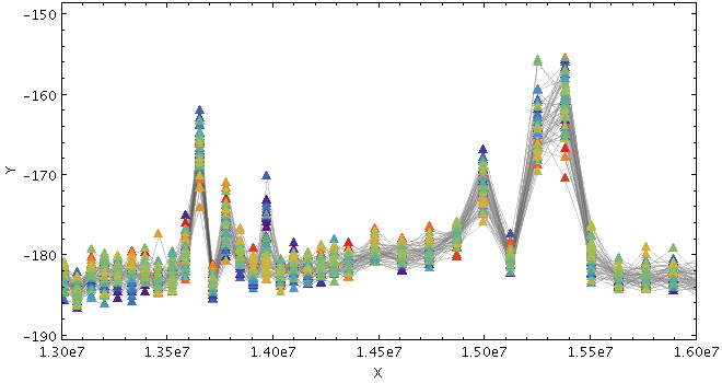
   stilts plot2plane in=LRS_NPW_V010_20071101.cdf xs=param$frequency ys=RX2
                     layer1=lines shading1=density densemap1=greyscale denseclip1=0.2,0.7
                     layer2=marks shading2=weighted weight2=epoch shape2=filled_triangle_down size2=4
                     xmin=13e6 xmax=16e6 xpix=660 icmd='head 50' auxmap=sron auxvisible=false
icmdN = <cmds> (ProcessingStep[])
inN.
The value of this parameter is one or more of the filter
commands described in Section 6.1.
If more than one is given, they must be separated by
semicolon characters (";").
This parameter can be repeated multiple times on the same
command line to build up a list of processing steps.
The sequence of commands given in this way
defines the processing pipeline which is performed on the table.
Commands may alternatively be supplied in an external file,
by using the indirection character '@'.
Thus a value of "@filename"
causes the file filename to be read for a list
of filter commands to execute. The commands in the file
may be separated by newline characters and/or semicolons,
and lines which are blank or which start with a
'#' character are ignored.
A backslash character '\' at the end of a line
joins it with the following line.
ifmtN = <in-format> (String)
inN.
The known formats are listed in Section 5.1.1.
This flag can be used if you know what format your
table is in.
If it has the special value
(auto) (the default),
then an attempt will be
made to detect the format of the table automatically.
This cannot always be done correctly however, in which case
the program will exit with an error explaining which
formats were attempted.
This parameter is ignored for scheme-specified tables.
[Default: (auto)]
inN = <table> (StarTable)
-",
meaning standard input.
In this case the input format must be given explicitly
using the ifmtN
parameter.
Note that not all formats can be streamed in this way.:<scheme-name>:<scheme-args>.<" character at the start,
or a "|" character at the end
("<syscmd" or
"syscmd|").
This executes the given pipeline and reads from its
standard output.
This will probably only work on unix-like systems.istreamN = true|false (Boolean)
inN parameter
will be read as a stream.
It is necessary to give the
ifmtN parameter
in this case.
Depending on the required operations and processing mode,
this may cause the read to fail (sometimes it is necessary
to read the table more than once).
It is not normally necessary to set this flag;
in most cases the data will be streamed automatically
if that is the best thing to do.
However it can sometimes result in less resource usage when
processing large files in certain formats (such as VOTable).
This parameter is ignored for scheme-specified tables.
[Default: false]
shadingN = auto|flat|translucent|transparent|density|aux|weighted|paux|pweighted <shade-paramsN> (ShapeMode)
[Default: auto]
shapeN = filled_circle|open_circle|... (MarkerShape)
The available options are:
filled_circle
open_circle
cross
x
open_square
open_diamond
open_triangle_up
open_triangle_down
fat_circle
fat_cross
fat_x
fat_square
fat_diamond
fat_triangle_up
fat_triangle_down
filled_square
filled_diamond
filled_triangle_up
filled_triangle_down
[Default: filled_circle]
sizeN = <pixels> (Integer)
[Default: 1]
xsN = <array-expr> (String)
The value is an array-valued algebraic expression based on column names as described in Section 10. Some of the functions in the Arrays class may be useful here.
ysN = <array-expr> (String)
The value is an array-valued algebraic expression based on column names as described in Section 10. Some of the functions in the Arrays class may be useful here.
handles
Draws a symbol representing the position of an X/Y array plot. Although this may not do a good job of showing the position for a whole X/Y array, which is line-like rather than point-like, it provides a visible reference position for the plotted row.
This plot type is therefore mostly useful in interactive environments like TOPCAT, where the plotted marker can be used for activating or identifying the corresponding table row.
Usage Overview:
   layerN=handles placementN=index|ymax|ymin|xmax|xmin|xymean fractionN=<0..1>
                  sizeN=<pixels> shapeN=filled_circle|open_circle|...
                  shadingN=auto|flat|translucent|transparent|density|aux|weighted|paux|pweighted <shade-paramsN>
                  xsN=<array-expr> ysN=<array-expr> inN=<table>
                  ifmtN=<in-format> istreamN=true|false icmdN=<cmds>
All the parameters listed here
affect only the relevant layer,
identified by the suffix
N.
Example:
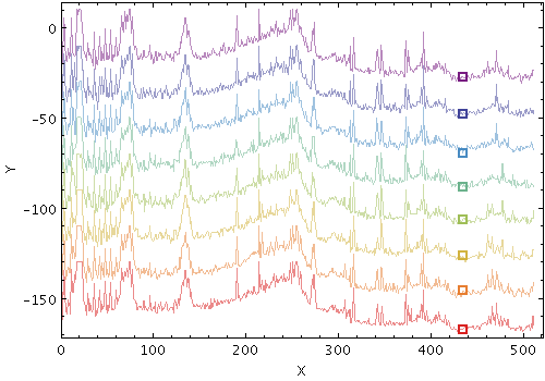
   stilts plot2plane in=LRS_NPW_V010_20071101.cdf ys=add(RX1,20*$index)
                     shading=aux auxmap=sron aux=$index
                     icmd='head 8' auxvisible=false legend=false
                     layer0=lines opaque0=2
                     layer1=handles placement1=index fraction1=0.85
fractionN = <0..1> (Double)
placement=index,
where it indicates how far through the array
the reference (X,Y) position should be taken
(0.0 means the first element, 1.0 means the last).
For other values of
placement
it is ignored.
[Default: 0.5]
icmdN = <cmds> (ProcessingStep[])
inN.
The value of this parameter is one or more of the filter
commands described in Section 6.1.
If more than one is given, they must be separated by
semicolon characters (";").
This parameter can be repeated multiple times on the same
command line to build up a list of processing steps.
The sequence of commands given in this way
defines the processing pipeline which is performed on the table.
Commands may alternatively be supplied in an external file,
by using the indirection character '@'.
Thus a value of "@filename"
causes the file filename to be read for a list
of filter commands to execute. The commands in the file
may be separated by newline characters and/or semicolons,
and lines which are blank or which start with a
'#' character are ignored.
A backslash character '\' at the end of a line
joins it with the following line.
ifmtN = <in-format> (String)
inN.
The known formats are listed in Section 5.1.1.
This flag can be used if you know what format your
table is in.
If it has the special value
(auto) (the default),
then an attempt will be
made to detect the format of the table automatically.
This cannot always be done correctly however, in which case
the program will exit with an error explaining which
formats were attempted.
This parameter is ignored for scheme-specified tables.
[Default: (auto)]
inN = <table> (StarTable)
-",
meaning standard input.
In this case the input format must be given explicitly
using the ifmtN
parameter.
Note that not all formats can be streamed in this way.:<scheme-name>:<scheme-args>.<" character at the start,
or a "|" character at the end
("<syscmd" or
"syscmd|").
This executes the given pipeline and reads from its
standard output.
This will probably only work on unix-like systems.istreamN = true|false (Boolean)
inN parameter
will be read as a stream.
It is necessary to give the
ifmtN parameter
in this case.
Depending on the required operations and processing mode,
this may cause the read to fail (sometimes it is necessary
to read the table more than once).
It is not normally necessary to set this flag;
in most cases the data will be streamed automatically
if that is the best thing to do.
However it can sometimes result in less resource usage when
processing large files in certain formats (such as VOTable).
This parameter is ignored for scheme-specified tables.
[Default: false]
placementN = index|ymax|ymin|xmax|xmin|xymean (XYArrayPlacement)
The available options are:
index: (X,Y) point at a certain fraction of the way through the arrays, as given by the fraction value; fraction=0.0 is the first element, fraction=1.0 is the last.ymax: (X,Y) position at which the maximum Y value is located (fraction is ignored)ymin: (X,Y) position at which the minimum Y value is located (fraction is ignored)xmax: (X,Y) position at which the maximum X value is located (fraction is ignored)xmin: (X,Y) position at which the minimum X value is located (fraction is ignored)xymean: center of gravity of all the (X,Y) points (fraction is ignored)[Default: index]
shadingN = auto|flat|translucent|transparent|density|aux|weighted|paux|pweighted <shade-paramsN> (ShapeMode)
[Default: auto]
shapeN = filled_circle|open_circle|... (MarkerShape)
The available options are:
filled_circle
open_circle
cross
x
open_square
open_diamond
open_triangle_up
open_triangle_down
fat_circle
fat_cross
fat_x
fat_square
fat_diamond
fat_triangle_up
fat_triangle_down
filled_square
filled_diamond
filled_triangle_up
filled_triangle_down
[Default: fat_square]
sizeN = <pixels> (Integer)
[Default: 4]
xsN = <array-expr> (String)
The value is an array-valued algebraic expression based on column names as described in Section 10. Some of the functions in the Arrays class may be useful here.
ysN = <array-expr> (String)
The value is an array-valued algebraic expression based on column names as described in Section 10. Some of the functions in the Arrays class may be useful here.
yerrors
Plots N error bars in the Y direction for each input row, with the X, Y and error bar extents each supplied by N-element array values.
Usage Overview:
   layerN=yerrors errorbarN=none|lines|capped_lines|caps|arrows
                  thickN=<int-value>
                  shadingN=auto|flat|translucent|transparent|density|aux|weighted|paux|pweighted <shade-paramsN>
                  xsN=<array-expr> ysN=<array-expr> yerrhisN=<array-expr>
                  yerrlosN=<array-expr> inN=<table> ifmtN=<in-format>
                  istreamN=true|false icmdN=<cmds>
All the parameters listed here
affect only the relevant layer,
identified by the suffix
N.
Example:
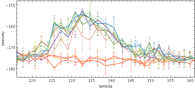
   stilts plot2plane in=LRS_NPW_V010_20071101.cdf
                     shading=aux aux=epoch
                     xs=divide(2.998e8,param$Frequency) ys=multiply(add(RX1,RX2),0.5)
                     layer_l=lines thick_l=2
                     layer_e=yerrors yerrhis_e=arrayFunc("abs(x)",subtract(RX1,RX2)) errorbar_e=capped_lines
                     auxmap=paired auxvisible=false
                     xmin=116 xmax=161 ymin=-184 ymax=-148 xpix=660 ypix=300 icmd='every 1000'
                     xlabel=lambda ylabel=Intensity
errorbarN = none|lines|capped_lines|caps|arrows (MultiPointShape)
The available options are:
none
lines
capped_lines
caps
arrows
[Default: lines]
icmdN = <cmds> (ProcessingStep[])
inN.
The value of this parameter is one or more of the filter
commands described in Section 6.1.
If more than one is given, they must be separated by
semicolon characters (";").
This parameter can be repeated multiple times on the same
command line to build up a list of processing steps.
The sequence of commands given in this way
defines the processing pipeline which is performed on the table.
Commands may alternatively be supplied in an external file,
by using the indirection character '@'.
Thus a value of "@filename"
causes the file filename to be read for a list
of filter commands to execute. The commands in the file
may be separated by newline characters and/or semicolons,
and lines which are blank or which start with a
'#' character are ignored.
A backslash character '\' at the end of a line
joins it with the following line.
ifmtN = <in-format> (String)
inN.
The known formats are listed in Section 5.1.1.
This flag can be used if you know what format your
table is in.
If it has the special value
(auto) (the default),
then an attempt will be
made to detect the format of the table automatically.
This cannot always be done correctly however, in which case
the program will exit with an error explaining which
formats were attempted.
This parameter is ignored for scheme-specified tables.
[Default: (auto)]
inN = <table> (StarTable)
-",
meaning standard input.
In this case the input format must be given explicitly
using the ifmtN
parameter.
Note that not all formats can be streamed in this way.:<scheme-name>:<scheme-args>.<" character at the start,
or a "|" character at the end
("<syscmd" or
"syscmd|").
This executes the given pipeline and reads from its
standard output.
This will probably only work on unix-like systems.istreamN = true|false (Boolean)
inN parameter
will be read as a stream.
It is necessary to give the
ifmtN parameter
in this case.
Depending on the required operations and processing mode,
this may cause the read to fail (sometimes it is necessary
to read the table more than once).
It is not normally necessary to set this flag;
in most cases the data will be streamed automatically
if that is the best thing to do.
However it can sometimes result in less resource usage when
processing large files in certain formats (such as VOTable).
This parameter is ignored for scheme-specified tables.
[Default: false]
shadingN = auto|flat|translucent|transparent|density|aux|weighted|paux|pweighted <shade-paramsN> (ShapeMode)
[Default: auto]
thickN = <int-value> (Integer)
[Default: 0]
xsN = <array-expr> (String)
The value is an array-valued algebraic expression based on column names as described in Section 10. Some of the functions in the Arrays class may be useful here.
yerrhisN = <array-expr> (String)
The value is an array-valued algebraic expression based on column names as described in Section 10. Some of the functions in the Arrays class may be useful here.
yerrlosN = <array-expr> (String)
The value is an array-valued algebraic expression based on column names as described in Section 10. Some of the functions in the Arrays class may be useful here.
ysN = <array-expr> (String)
The value is an array-valued algebraic expression based on column names as described in Section 10. Some of the functions in the Arrays class may be useful here.
xyerrors
Plots N error bars in the X and Y directions for each input row, with the X, Y and error bar extents each supplied by N-element array values.
Usage Overview:
   layerN=xyerrors errorbarN=none|lines|capped_lines|... thickN=<int-value>
                   shadingN=auto|flat|translucent|transparent|density|aux|weighted|paux|pweighted <shade-paramsN>
                   xsN=<array-expr> ysN=<array-expr> xerrhisN=<array-expr>
                   xerrlosN=<array-expr> yerrhisN=<array-expr>
                   yerrlosN=<array-expr> inN=<table> ifmtN=<in-format>
                   istreamN=true|false icmdN=<cmds>
All the parameters listed here
affect only the relevant layer,
identified by the suffix
N.
Example:
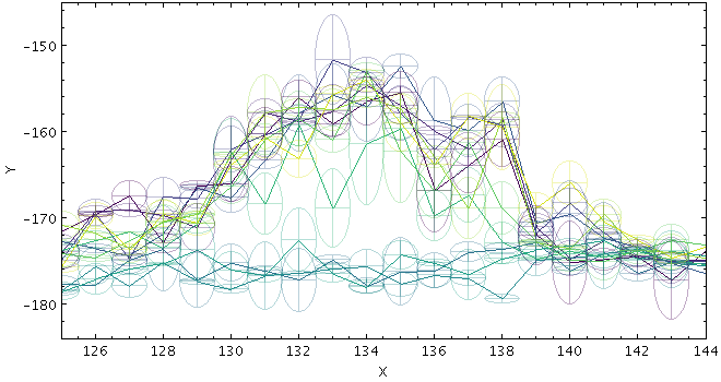
   stilts plot2plane in=LRS_NPW_V010_20071101.cdf ys=RX1
                     shading=aux aux=epoch
                     layer_l=lines opaque_l=1
                     layer_xy=xyerrors opaque_xy=3.3 errorbar_xy=crosshair_ellipse
                     xerrhis_xy=constant(512,0.5) yerrhis_xy=arrayFunc("abs(x)",subtract(RX1,RX2))
                     xmin=125 xmax=144 ymin=-184 ymax=-145 xpix=660 icmd='every 1000'
                     auxmap=viridis auxvisible=false
errorbarN = none|lines|capped_lines|... (MultiPointShape)
The available options are:
none
lines
capped_lines
caps
arrows
ellipse
crosshair_ellipse
rectangle
crosshair_rectangle
filled_ellipse
filled_rectangle
[Default: lines]
icmdN = <cmds> (ProcessingStep[])
inN.
The value of this parameter is one or more of the filter
commands described in Section 6.1.
If more than one is given, they must be separated by
semicolon characters (";").
This parameter can be repeated multiple times on the same
command line to build up a list of processing steps.
The sequence of commands given in this way
defines the processing pipeline which is performed on the table.
Commands may alternatively be supplied in an external file,
by using the indirection character '@'.
Thus a value of "@filename"
causes the file filename to be read for a list
of filter commands to execute. The commands in the file
may be separated by newline characters and/or semicolons,
and lines which are blank or which start with a
'#' character are ignored.
A backslash character '\' at the end of a line
joins it with the following line.
ifmtN = <in-format> (String)
inN.
The known formats are listed in Section 5.1.1.
This flag can be used if you know what format your
table is in.
If it has the special value
(auto) (the default),
then an attempt will be
made to detect the format of the table automatically.
This cannot always be done correctly however, in which case
the program will exit with an error explaining which
formats were attempted.
This parameter is ignored for scheme-specified tables.
[Default: (auto)]
inN = <table> (StarTable)
-",
meaning standard input.
In this case the input format must be given explicitly
using the ifmtN
parameter.
Note that not all formats can be streamed in this way.:<scheme-name>:<scheme-args>.<" character at the start,
or a "|" character at the end
("<syscmd" or
"syscmd|").
This executes the given pipeline and reads from its
standard output.
This will probably only work on unix-like systems.istreamN = true|false (Boolean)
inN parameter
will be read as a stream.
It is necessary to give the
ifmtN parameter
in this case.
Depending on the required operations and processing mode,
this may cause the read to fail (sometimes it is necessary
to read the table more than once).
It is not normally necessary to set this flag;
in most cases the data will be streamed automatically
if that is the best thing to do.
However it can sometimes result in less resource usage when
processing large files in certain formats (such as VOTable).
This parameter is ignored for scheme-specified tables.
[Default: false]
shadingN = auto|flat|translucent|transparent|density|aux|weighted|paux|pweighted <shade-paramsN> (ShapeMode)
[Default: auto]
thickN = <int-value> (Integer)
[Default: 0]
xerrhisN = <array-expr> (String)
The value is an array-valued algebraic expression based on column names as described in Section 10. Some of the functions in the Arrays class may be useful here.
xerrlosN = <array-expr> (String)
The value is an array-valued algebraic expression based on column names as described in Section 10. Some of the functions in the Arrays class may be useful here.
xsN = <array-expr> (String)
The value is an array-valued algebraic expression based on column names as described in Section 10. Some of the functions in the Arrays class may be useful here.
yerrhisN = <array-expr> (String)
The value is an array-valued algebraic expression based on column names as described in Section 10. Some of the functions in the Arrays class may be useful here.
yerrlosN = <array-expr> (String)
The value is an array-valued algebraic expression based on column names as described in Section 10. Some of the functions in the Arrays class may be useful here.
ysN = <array-expr> (String)
The value is an array-valued algebraic expression based on column names as described in Section 10. Some of the functions in the Arrays class may be useful here.
statline
Plots a single line based on a combination (typically the mean) of input array-valued coordinates. The input X and Y coordinates must be fixed-length arrays of length N; a line with N points is plotted, each point representing the mean (or median, minimum, maximum, ...) of all the input array elements at the corresponding position.
Note that because the X and Y arrays must be of a fixed size for all rows, and because combination is performed in both X and Y directions, this is typically only suitable for plotting combined spectra if they all share a common horizontal axis, e.g. are all sampled into the same wavelength bins. To visually combine spectra with non-uniform sampling, the arrayquantile plotter may be more useful.
Usage Overview:
   layerN=statline xcombineN=mean|median|min|max|q.01|...
                   ycombineN=mean|median|min|max|q.01|...
                   colorN=<rrggbb>|red|blue|... thickN=<pixels>
                   antialiasN=true|false xsN=<array-expr> ysN=<array-expr>
                   inN=<table> ifmtN=<in-format> istreamN=true|false
                   icmdN=<cmds>
All the parameters listed here
affect only the relevant layer,
identified by the suffix
N.
Example:
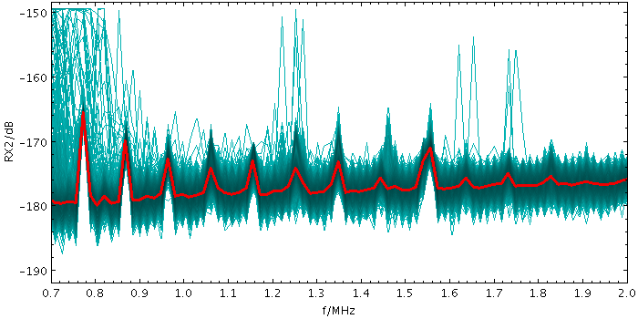
   stilts plot2plane in=LRS_NPW_V010_20071101.cdf xs=multiply(param$frequency,1e-6) ys=RX2
                     xlabel=f/MHz ylabel=RX2/dB xmin=0.7 xmax=2.0 icmd='select rx2[71]<-170' xpix=700
                     layer1=lines color1=cyan
                     layer2=statline color2=red thick2=3
antialiasN = true|false (Boolean)
[Default: false]
colorN = <rrggbb>|red|blue|... (Color)
The standard plotting colour names are
red, blue, green, grey, magenta, cyan, orange, pink, yellow, black, light_grey, white.
However, many other common colour names (too many to list here)
are also understood.
The list currently contains those colour names understood
by most web browsers,
from AliceBlue to YellowGreen,
listed e.g. in the
Extended color keywords section of
the CSS3 standard.
Alternatively, a six-digit hexadecimal number RRGGBB
may be supplied,
optionally prefixed by "#" or "0x",
giving red, green and blue intensities,
e.g. "ff00ff", "#ff00ff"
or "0xff00ff" for magenta.
[Default: red]
icmdN = <cmds> (ProcessingStep[])
inN.
The value of this parameter is one or more of the filter
commands described in Section 6.1.
If more than one is given, they must be separated by
semicolon characters (";").
This parameter can be repeated multiple times on the same
command line to build up a list of processing steps.
The sequence of commands given in this way
defines the processing pipeline which is performed on the table.
Commands may alternatively be supplied in an external file,
by using the indirection character '@'.
Thus a value of "@filename"
causes the file filename to be read for a list
of filter commands to execute. The commands in the file
may be separated by newline characters and/or semicolons,
and lines which are blank or which start with a
'#' character are ignored.
A backslash character '\' at the end of a line
joins it with the following line.
ifmtN = <in-format> (String)
inN.
The known formats are listed in Section 5.1.1.
This flag can be used if you know what format your
table is in.
If it has the special value
(auto) (the default),
then an attempt will be
made to detect the format of the table automatically.
This cannot always be done correctly however, in which case
the program will exit with an error explaining which
formats were attempted.
This parameter is ignored for scheme-specified tables.
[Default: (auto)]
inN = <table> (StarTable)
-",
meaning standard input.
In this case the input format must be given explicitly
using the ifmtN
parameter.
Note that not all formats can be streamed in this way.:<scheme-name>:<scheme-args>.<" character at the start,
or a "|" character at the end
("<syscmd" or
"syscmd|").
This executes the given pipeline and reads from its
standard output.
This will probably only work on unix-like systems.istreamN = true|false (Boolean)
inN parameter
will be read as a stream.
It is necessary to give the
ifmtN parameter
in this case.
Depending on the required operations and processing mode,
this may cause the read to fail (sometimes it is necessary
to read the table more than once).
It is not normally necessary to set this flag;
in most cases the data will be streamed automatically
if that is the best thing to do.
However it can sometimes result in less resource usage when
processing large files in certain formats (such as VOTable).
This parameter is ignored for scheme-specified tables.
[Default: false]
thickN = <pixels> (Integer)
[Default: 3]
xcombineN = mean|median|min|max|q.01|... (Combiner)
The available options are:
mean: the mean of the combined valuesmedian: the medianmin: the minimum of all the combined valuesmax: the maximum of all the combined valuesq.01: 1st percentileq1: first quartileq3: third quartileq.99: 99th percentilestdev: the sample standard deviation of the combined valuessum: the sum of all the combined values per bincount: the number of non-blank values per bin (weight is ignored)[Default: mean]
xsN = <array-expr> (String)
The value is an array-valued algebraic expression based on column names as described in Section 10. Some of the functions in the Arrays class may be useful here.
ycombineN = mean|median|min|max|q.01|... (Combiner)
The available options are:
mean: the mean of the combined valuesmedian: the medianmin: the minimum of all the combined valuesmax: the maximum of all the combined valuesq.01: 1st percentileq1: first quartileq3: third quartileq.99: 99th percentilestdev: the sample standard deviation of the combined valuessum: the sum of all the combined values per bincount: the number of non-blank values per bin (weight is ignored)[Default: mean]
ysN = <array-expr> (String)
The value is an array-valued algebraic expression based on column names as described in Section 10. Some of the functions in the Arrays class may be useful here.
statmark
Plots a set of markers based on a combination (typically the mean) of input array-valued coordinates. The input X and Y coordinates must be fixed-length arrays of length N; N markers are plotted, each one representing the mean (or median, minimum, maximum, ...) of all the input array elements at the corresponding position.
Note that because the X and Y arrays must be of a fixed size for all rows, and because combination is performed in both X and Y directions, this is typically only suitable for plotting combined spectra if they all share a common horizontal axis, e.g. are all sampled into the same wavelength bins. To visually combine spectra with non-uniform sampling, the arrayquantile plotter may be more useful.
Usage Overview:
   layerN=statmark xcombineN=mean|median|min|max|q.01|...
                   ycombineN=mean|median|min|max|q.01|...
                   colorN=<rrggbb>|red|blue|...
                   shapeN=filled_circle|open_circle|... sizeN=<pixels>
                   xsN=<array-expr> ysN=<array-expr> inN=<table>
                   ifmtN=<in-format> istreamN=true|false icmdN=<cmds>
All the parameters listed here
affect only the relevant layer,
identified by the suffix
N.
Example:
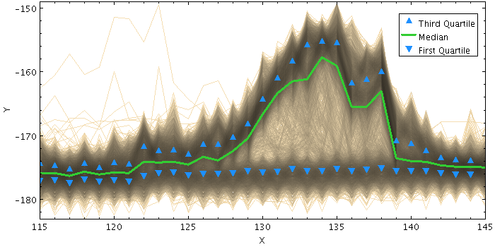
   stilts plot2plane in=LRS_NPW_V010_20071101.cdf ys=RX1
                     xmin=115 xmax=145 ymin=-183 ymax=-149 xpix=700 xcrowd=0.8
                     layer-d=lines color-d=wheat
                     layer-m=statline ycombine-m=median color-m=LimeGreen thick-m=3
                     color-q=DodgerBlue size-q=4
                     layer-q1=statmark ycombine-q1=Q1 shape-q1=filled_triangle_up
                     layer-q3=statmark ycombine-q3=Q3 shape-q3=filled_triangle_down
                     leglabel-m=Median leglabel-q1='First Quartile' leglabel-q3='Third Quartile'
                     legseq=-q3,-m,-q1 legpos=0.98,0.93
colorN = <rrggbb>|red|blue|... (Color)
The standard plotting colour names are
red, blue, green, grey, magenta, cyan, orange, pink, yellow, black, light_grey, white.
However, many other common colour names (too many to list here)
are also understood.
The list currently contains those colour names understood
by most web browsers,
from AliceBlue to YellowGreen,
listed e.g. in the
Extended color keywords section of
the CSS3 standard.
Alternatively, a six-digit hexadecimal number RRGGBB
may be supplied,
optionally prefixed by "#" or "0x",
giving red, green and blue intensities,
e.g. "ff00ff", "#ff00ff"
or "0xff00ff" for magenta.
[Default: red]
icmdN = <cmds> (ProcessingStep[])
inN.
The value of this parameter is one or more of the filter
commands described in Section 6.1.
If more than one is given, they must be separated by
semicolon characters (";").
This parameter can be repeated multiple times on the same
command line to build up a list of processing steps.
The sequence of commands given in this way
defines the processing pipeline which is performed on the table.
Commands may alternatively be supplied in an external file,
by using the indirection character '@'.
Thus a value of "@filename"
causes the file filename to be read for a list
of filter commands to execute. The commands in the file
may be separated by newline characters and/or semicolons,
and lines which are blank or which start with a
'#' character are ignored.
A backslash character '\' at the end of a line
joins it with the following line.
ifmtN = <in-format> (String)
inN.
The known formats are listed in Section 5.1.1.
This flag can be used if you know what format your
table is in.
If it has the special value
(auto) (the default),
then an attempt will be
made to detect the format of the table automatically.
This cannot always be done correctly however, in which case
the program will exit with an error explaining which
formats were attempted.
This parameter is ignored for scheme-specified tables.
[Default: (auto)]
inN = <table> (StarTable)
-",
meaning standard input.
In this case the input format must be given explicitly
using the ifmtN
parameter.
Note that not all formats can be streamed in this way.:<scheme-name>:<scheme-args>.<" character at the start,
or a "|" character at the end
("<syscmd" or
"syscmd|").
This executes the given pipeline and reads from its
standard output.
This will probably only work on unix-like systems.istreamN = true|false (Boolean)
inN parameter
will be read as a stream.
It is necessary to give the
ifmtN parameter
in this case.
Depending on the required operations and processing mode,
this may cause the read to fail (sometimes it is necessary
to read the table more than once).
It is not normally necessary to set this flag;
in most cases the data will be streamed automatically
if that is the best thing to do.
However it can sometimes result in less resource usage when
processing large files in certain formats (such as VOTable).
This parameter is ignored for scheme-specified tables.
[Default: false]
shapeN = filled_circle|open_circle|... (MarkerShape)
The available options are:
filled_circle
open_circle
cross
x
open_square
open_diamond
open_triangle_up
open_triangle_down
fat_circle
fat_cross
fat_x
fat_square
fat_diamond
fat_triangle_up
fat_triangle_down
filled_square
filled_diamond
filled_triangle_up
filled_triangle_down
[Default: filled_circle]
sizeN = <pixels> (Integer)
[Default: 4]
xcombineN = mean|median|min|max|q.01|... (Combiner)
The available options are:
mean: the mean of the combined valuesmedian: the medianmin: the minimum of all the combined valuesmax: the maximum of all the combined valuesq.01: 1st percentileq1: first quartileq3: third quartileq.99: 99th percentilestdev: the sample standard deviation of the combined valuessum: the sum of all the combined values per bincount: the number of non-blank values per bin (weight is ignored)[Default: mean]
xsN = <array-expr> (String)
The value is an array-valued algebraic expression based on column names as described in Section 10. Some of the functions in the Arrays class may be useful here.
ycombineN = mean|median|min|max|q.01|... (Combiner)
The available options are:
mean: the mean of the combined valuesmedian: the medianmin: the minimum of all the combined valuesmax: the maximum of all the combined valuesq.01: 1st percentileq1: first quartileq3: third quartileq.99: 99th percentilestdev: the sample standard deviation of the combined valuessum: the sum of all the combined values per bincount: the number of non-blank values per bin (weight is ignored)[Default: mean]
ysN = <array-expr> (String)
The value is an array-valued algebraic expression based on column names as described in Section 10. Some of the functions in the Arrays class may be useful here.
arrayquantile
Displays a quantile or quantile range for a set of plotted X/Y array pairs. If a table contains one spectrum per row in array-valued wavelength and flux columns, this plotter can be used to display a median of all the spectra, or a range between two quantiles. Smoothing options are available to even out noise arising from the pixel binning.
For each row, the
xs and
ys arrays
must be the same length as each other,
but this plot type does not require all the arrays
to be sampled into the same bins.
The algorithm calculates quantiles for all the X,Y points plotted in each column of pixels. This means that more densely sampled spectra have more influence on the output than sparser ones.
Note: in the current implementation, depending on the details of the configuration and the data, there may be some distortions or missing graphics near the edges of the plot. This may be improved in future releases, depending on feedback.
Usage Overview:
   layerN=arrayquantile colorN=<rrggbb>|red|blue|... transparencyN=0..1
                        quantilesN=<low-frac>[,<high-frac>] thickN=<pixels>
                        smoothN=+<width>|-<count>
                        kernelN=square|linear|epanechnikov|cos|cos2|gauss3|gauss6
                        joinN=none|polygon|lines horizontalN=true|false
                        xsN=<array-expr> ysN=<array-expr> inN=<table>
                        ifmtN=<in-format> istreamN=true|false icmdN=<cmds>
All the parameters listed here
affect only the relevant layer,
identified by the suffix
N.
Example:
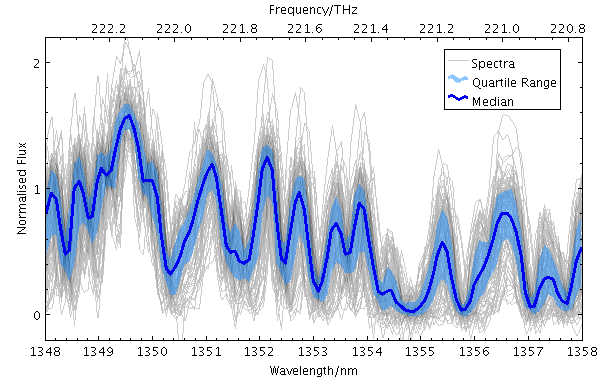
   stilts plot2plane in=xq100sub.fits xs=subWave ys=multiply(subFlux,1./mean(subFlux))
                     xlabel=Wavelength/nm ylabel='Normalised Flux'
                     x2func=SPEED_OF_LIGHT*1E9*1E-12/x x2label=Frequency/THz
                     layer1=lines shading1=density densemap1=greyscale
                     denseclip1=0.2,1 densefunc1=linear leglabel1=Spectra
                     layer_q13=ArrayQuantile color_q13=DodgerBlue transparency_q13=0.5
                     quantiles_q13=0.25,0.75 leglabel_q13='Quartile Range'
                     layer_med=ArrayQuantile color_med=blue join_med=lines leglabel_med=Median
                     legend=true legpos=0.95,0.95
                     xpix=600 ypix=380
                     xmin=1348 xmax=1358 ymin=-0.2 ymax=2.2
colorN = <rrggbb>|red|blue|... (Color)
The standard plotting colour names are
red, blue, green, grey, magenta, cyan, orange, pink, yellow, black, light_grey, white.
However, many other common colour names (too many to list here)
are also understood.
The list currently contains those colour names understood
by most web browsers,
from AliceBlue to YellowGreen,
listed e.g. in the
Extended color keywords section of
the CSS3 standard.
Alternatively, a six-digit hexadecimal number RRGGBB
may be supplied,
optionally prefixed by "#" or "0x",
giving red, green and blue intensities,
e.g. "ff00ff", "#ff00ff"
or "0xff00ff" for magenta.
[Default: red]
horizontalN = true|false (Boolean)
true, y quantiles are calculated
for each pixel column, and
if false, x quantiles are calculated
for each pixel row.
[Default: true]
icmdN = <cmds> (ProcessingStep[])
inN.
The value of this parameter is one or more of the filter
commands described in Section 6.1.
If more than one is given, they must be separated by
semicolon characters (";").
This parameter can be repeated multiple times on the same
command line to build up a list of processing steps.
The sequence of commands given in this way
defines the processing pipeline which is performed on the table.
Commands may alternatively be supplied in an external file,
by using the indirection character '@'.
Thus a value of "@filename"
causes the file filename to be read for a list
of filter commands to execute. The commands in the file
may be separated by newline characters and/or semicolons,
and lines which are blank or which start with a
'#' character are ignored.
A backslash character '\' at the end of a line
joins it with the following line.
ifmtN = <in-format> (String)
inN.
The known formats are listed in Section 5.1.1.
This flag can be used if you know what format your
table is in.
If it has the special value
(auto) (the default),
then an attempt will be
made to detect the format of the table automatically.
This cannot always be done correctly however, in which case
the program will exit with an error explaining which
formats were attempted.
This parameter is ignored for scheme-specified tables.
[Default: (auto)]
inN = <table> (StarTable)
-",
meaning standard input.
In this case the input format must be given explicitly
using the ifmtN
parameter.
Note that not all formats can be streamed in this way.:<scheme-name>:<scheme-args>.<" character at the start,
or a "|" character at the end
("<syscmd" or
"syscmd|").
This executes the given pipeline and reads from its
standard output.
This will probably only work on unix-like systems.istreamN = true|false (Boolean)
inN parameter
will be read as a stream.
It is necessary to give the
ifmtN parameter
in this case.
Depending on the required operations and processing mode,
this may cause the read to fail (sometimes it is necessary
to read the table more than once).
It is not normally necessary to set this flag;
in most cases the data will be streamed automatically
if that is the best thing to do.
However it can sometimes result in less resource usage when
processing large files in certain formats (such as VOTable).
This parameter is ignored for scheme-specified tables.
[Default: false]
joinN = none|polygon|lines (QJoin)
The available options are:
none: displayed quantile ranges are not joinedpolygon: the area between a line connecting the upper quantiles and a line connecting the lower quantiles is filledlines: a line of thickness given by thick is drawn from the center of each quantile range to the next[Default: polygon]
kernelN = square|linear|epanechnikov|cos|cos2|gauss3|gauss6 (Kernel1dShape)
The available options are:
square: Uniform value: f(x)=1, |x|=0..1linear: Triangle: f(x)=1-|x|, |x|=0..1epanechnikov: Parabola: f(x)=1-x*x, |x|=0..1cos: Cosine: f(x)=cos(x*pi/2), |x|=0..1cos2: Cosine squared: f(x)=cos^2(x*pi/2), |x|=0..1gauss3: Gaussian truncated at 3.0 sigma: f(x)=exp(-x*x/2), |x|=0..3gauss6: Gaussian truncated at 6.0 sigma: f(x)=exp(-x*x/2), |x|=0..6[Default: epanechnikov]
quantilesN = <low-frac>[,<high-frac>] (Subrange)
<lo>,<hi>)
indicating two quantile lines bounding an area to be filled.
A pair of equal values "a,a"
is equivalent to the single value "a".
The default is 0.5,
which means to mark the median value in each column,
and could equivalently be specified 0.5,0.5.
[Default: 0.5]
smoothN = +<width>|-<count> (BinSizer)
If the supplied value is a positive number it is interpreted as a fixed width in the data coordinates of the X axis (if the X axis is logarithmic, the value is a fixed factor). If it is a negative number, then it will be interpreted as the approximate number of smooothing widths that fit in the width of the visible plot (i.e. plot width / smoothing width). If the value is zero, no smoothing is applied.
When setting this value graphically, you can use either the slider to adjust the bin count or the numeric entry field to fix the bin width.
[Default: 0]
thickN = <pixels> (Integer)
quantiles
specifies a single value rather than a pair)
this will give the actual thickness of the plotted line.
If the range is non-zero however, the line may be thicker
than this in places according to the quantile positions.
[Default: 3]
transparencyN = 0..1 (Double)
[Default: 0]
xsN = <array-expr> (String)
The value is an array-valued algebraic expression based on column names as described in Section 10. Some of the functions in the Arrays class may be useful here.
ysN = <array-expr> (String)
The value is an array-valued algebraic expression based on column names as described in Section 10. Some of the functions in the Arrays class may be useful here.
line
Plots a point-to-point line joining
up the positions of data points.
There are additional options to pre-sort the points
according to their order on the X or Y axis (using the
sortaxis
value),
and to vary the colour of the line along its length (using the
aux
value).
The options for controlling the Aux colour map are controlled at the level of the plot itself, rather than by per-layer configuration.
Usage Overview:
   layerN=line colorN=<rrggbb>|red|blue|... thickN=<pixels>
               dashN=dot|dash|...|<a,b,...> sortaxisN=[X|Y]
               antialiasN=true|false auxnullcolorN=<rrggbb>|red|blue|...
               <pos-coord-paramsN> auxN=<num-expr> inN=<table>
               ifmtN=<in-format> istreamN=true|false icmdN=<cmds>
All the parameters listed here
affect only the relevant layer,
identified by the suffix
N.
<pos-coord-paramsN>
give a position for each row of the input table.
Their form depends on the plot geometry,
i.e. which plotting command is used.
For a plane plot (plot2plane)
the parameters would be
xN and yN.
The coordinate parameter values are in all cases strings
interpreted as numeric expressions based on column names.
These can be column names, fixed values or algebraic
expressions as described in Section 10.
Example:
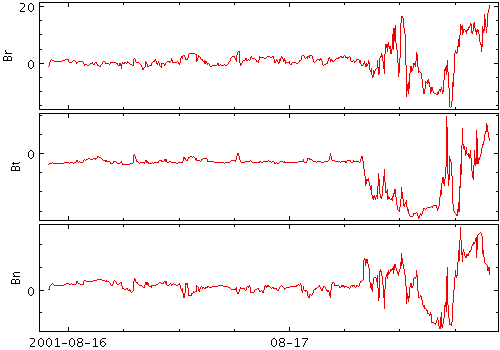
   stilts plot2time in=ACE_data.vot t=epoch
                    layer1=line y1=Br zone1=A
                    layer2=line y2=Bt zone2=B
                    layer3=line y3=Bn zone3=C
antialiasN = true|false (Boolean)
[Default: false]
auxN = <num-expr> (String)
The value is a numeric algebraic expression based on column names as described in Section 10.
auxnullcolorN = <rrggbb>|red|blue|... (Color)
The standard plotting colour names are
red, blue, green, grey, magenta, cyan, orange, pink, yellow, black, light_grey, white.
However, many other common colour names (too many to list here)
are also understood.
The list currently contains those colour names understood
by most web browsers,
from AliceBlue to YellowGreen,
listed e.g. in the
Extended color keywords section of
the CSS3 standard.
Alternatively, a six-digit hexadecimal number RRGGBB
may be supplied,
optionally prefixed by "#" or "0x",
giving red, green and blue intensities,
e.g. "ff00ff", "#ff00ff"
or "0xff00ff" for magenta.
If the value is null, then points with a null Aux value will not be plotted at all.
[Default: grey]
colorN = <rrggbb>|red|blue|... (Color)
The standard plotting colour names are
red, blue, green, grey, magenta, cyan, orange, pink, yellow, black, light_grey, white.
However, many other common colour names (too many to list here)
are also understood.
The list currently contains those colour names understood
by most web browsers,
from AliceBlue to YellowGreen,
listed e.g. in the
Extended color keywords section of
the CSS3 standard.
Alternatively, a six-digit hexadecimal number RRGGBB
may be supplied,
optionally prefixed by "#" or "0x",
giving red, green and blue intensities,
e.g. "ff00ff", "#ff00ff"
or "0xff00ff" for magenta.
[Default: red]
dashN = dot|dash|...|<a,b,...> (float[])
Possible values for dashed lines are
dot, dash, longdash, dotdash.
You can alternatively supply a comma-separated list
of on/off length values such as
"4,2,8,2".
icmdN = <cmds> (ProcessingStep[])
inN.
The value of this parameter is one or more of the filter
commands described in Section 6.1.
If more than one is given, they must be separated by
semicolon characters (";").
This parameter can be repeated multiple times on the same
command line to build up a list of processing steps.
The sequence of commands given in this way
defines the processing pipeline which is performed on the table.
Commands may alternatively be supplied in an external file,
by using the indirection character '@'.
Thus a value of "@filename"
causes the file filename to be read for a list
of filter commands to execute. The commands in the file
may be separated by newline characters and/or semicolons,
and lines which are blank or which start with a
'#' character are ignored.
A backslash character '\' at the end of a line
joins it with the following line.
ifmtN = <in-format> (String)
inN.
The known formats are listed in Section 5.1.1.
This flag can be used if you know what format your
table is in.
If it has the special value
(auto) (the default),
then an attempt will be
made to detect the format of the table automatically.
This cannot always be done correctly however, in which case
the program will exit with an error explaining which
formats were attempted.
This parameter is ignored for scheme-specified tables.
[Default: (auto)]
inN = <table> (StarTable)
-",
meaning standard input.
In this case the input format must be given explicitly
using the ifmtN
parameter.
Note that not all formats can be streamed in this way.:<scheme-name>:<scheme-args>.<" character at the start,
or a "|" character at the end
("<syscmd" or
"syscmd|").
This executes the given pipeline and reads from its
standard output.
This will probably only work on unix-like systems.istreamN = true|false (Boolean)
inN parameter
will be read as a stream.
It is necessary to give the
ifmtN parameter
in this case.
Depending on the required operations and processing mode,
this may cause the read to fail (sometimes it is necessary
to read the table more than once).
It is not normally necessary to set this flag;
in most cases the data will be streamed automatically
if that is the best thing to do.
However it can sometimes result in less resource usage when
processing large files in certain formats (such as VOTable).
This parameter is ignored for scheme-specified tables.
[Default: false]
sortaxisN = [X|Y] (AxisOpt)
X" or
"Y"
to ensure that the points are plotted in ascending order
of the corresponding coordinate.
This will ensure that the plotted line resembles a
function of the corresponding coordinate rather than
a scribble.
The default (null) value causes the points to be joined
in the sequence in which they appear in the table.
If the points already appear in the table sorted
according to the corresponding coordinate,
this option has no visible effect,
though it may slow things down.
[Default: None]
thickN = <pixels> (Integer)
[Default: 1]
linearfit
Plots a line of best fit for the data points.
Usage Overview:
   layerN=linearfit colorN=<rrggbb>|red|blue|... thickN=<pixels>
                    dashN=dot|dash|...|<a,b,...> antialiasN=true|false
                    <pos-coord-paramsN> weightN=<num-expr> inN=<table>
                    ifmtN=<in-format> istreamN=true|false icmdN=<cmds>
All the parameters listed here
affect only the relevant layer,
identified by the suffix
N.
<pos-coord-paramsN>
give a position for each row of the input table.
Their form depends on the plot geometry,
i.e. which plotting command is used.
For a plane plot (plot2plane)
the parameters would be
xN and yN.
The coordinate parameter values are in all cases strings
interpreted as numeric expressions based on column names.
These can be column names, fixed values or algebraic
expressions as described in Section 10.
Example:
stilts plot2plane in=6dfgs_mini.xml x=RMAG y=BMAG layer1=mark layer2=linearfit
antialiasN = true|false (Boolean)
[Default: false]
colorN = <rrggbb>|red|blue|... (Color)
The standard plotting colour names are
red, blue, green, grey, magenta, cyan, orange, pink, yellow, black, light_grey, white.
However, many other common colour names (too many to list here)
are also understood.
The list currently contains those colour names understood
by most web browsers,
from AliceBlue to YellowGreen,
listed e.g. in the
Extended color keywords section of
the CSS3 standard.
Alternatively, a six-digit hexadecimal number RRGGBB
may be supplied,
optionally prefixed by "#" or "0x",
giving red, green and blue intensities,
e.g. "ff00ff", "#ff00ff"
or "0xff00ff" for magenta.
[Default: red]
dashN = dot|dash|...|<a,b,...> (float[])
Possible values for dashed lines are
dot, dash, longdash, dotdash.
You can alternatively supply a comma-separated list
of on/off length values such as
"4,2,8,2".
icmdN = <cmds> (ProcessingStep[])
inN.
The value of this parameter is one or more of the filter
commands described in Section 6.1.
If more than one is given, they must be separated by
semicolon characters (";").
This parameter can be repeated multiple times on the same
command line to build up a list of processing steps.
The sequence of commands given in this way
defines the processing pipeline which is performed on the table.
Commands may alternatively be supplied in an external file,
by using the indirection character '@'.
Thus a value of "@filename"
causes the file filename to be read for a list
of filter commands to execute. The commands in the file
may be separated by newline characters and/or semicolons,
and lines which are blank or which start with a
'#' character are ignored.
A backslash character '\' at the end of a line
joins it with the following line.
ifmtN = <in-format> (String)
inN.
The known formats are listed in Section 5.1.1.
This flag can be used if you know what format your
table is in.
If it has the special value
(auto) (the default),
then an attempt will be
made to detect the format of the table automatically.
This cannot always be done correctly however, in which case
the program will exit with an error explaining which
formats were attempted.
This parameter is ignored for scheme-specified tables.
[Default: (auto)]
inN = <table> (StarTable)
-",
meaning standard input.
In this case the input format must be given explicitly
using the ifmtN
parameter.
Note that not all formats can be streamed in this way.:<scheme-name>:<scheme-args>.<" character at the start,
or a "|" character at the end
("<syscmd" or
"syscmd|").
This executes the given pipeline and reads from its
standard output.
This will probably only work on unix-like systems.istreamN = true|false (Boolean)
inN parameter
will be read as a stream.
It is necessary to give the
ifmtN parameter
in this case.
Depending on the required operations and processing mode,
this may cause the read to fail (sometimes it is necessary
to read the table more than once).
It is not normally necessary to set this flag;
in most cases the data will be streamed automatically
if that is the best thing to do.
However it can sometimes result in less resource usage when
processing large files in certain formats (such as VOTable).
This parameter is ignored for scheme-specified tables.
[Default: false]
thickN = <pixels> (Integer)
[Default: 1]
weightN = <num-expr> (String)
Given certain assumptions about independence of samples,
a suitable value for the weight may be
1/(err*err), if err is the
measurement error for each Y value.
The value is a numeric algebraic expression based on column names as described in Section 10.
label
Draws a text label at each position. You can select the font, where the labels appear in relation to the point positions, and how crowded the points have to get before they are suppressed.
Usage Overview:
   layerN=label texttypeN=plain|antialias|latex fontsizeN=<int-value>
                fontstyleN=standard|serif|mono
                fontweightN=plain|bold|italic|bold_italic
                anchorN=west|east|north|south|center
                colorN=<rrggbb>|red|blue|... xoffN=<pixels> yoffN=<pixels>
                spacingN=<pixels> crowdlimitN=<n> <pos-coord-paramsN>
                labelN=<txt-expr> inN=<table> ifmtN=<in-format>
                istreamN=true|false icmdN=<cmds>
All the parameters listed here
affect only the relevant layer,
identified by the suffix
N.
<pos-coord-paramsN>
give a position for each row of the input table.
Their form depends on the plot geometry,
i.e. which plotting command is used.
For a plane plot (plot2plane)
the parameters would be
xN and yN.
The coordinate parameter values are in all cases strings
interpreted as numeric expressions based on column names.
These can be column names, fixed values or algebraic
expressions as described in Section 10.
Example:
   stilts plot2sky in=messier.xml lon=RA lat=DEC
                   layer1=mark size1=3
                   layer2=label label2=NAME color2=black
anchorN = west|east|north|south|center (Anchor)
The available options are:
west
east
north
south
center
[Default: west]
colorN = <rrggbb>|red|blue|... (Color)
The standard plotting colour names are
red, blue, green, grey, magenta, cyan, orange, pink, yellow, black, light_grey, white.
However, many other common colour names (too many to list here)
are also understood.
The list currently contains those colour names understood
by most web browsers,
from AliceBlue to YellowGreen,
listed e.g. in the
Extended color keywords section of
the CSS3 standard.
Alternatively, a six-digit hexadecimal number RRGGBB
may be supplied,
optionally prefixed by "#" or "0x",
giving red, green and blue intensities,
e.g. "ff00ff", "#ff00ff"
or "0xff00ff" for magenta.
[Default: red]
crowdlimitN = <n> (Integer)
It is useful for instance if you are looking at pairs of points, which will always be close together; if you set this value to 2, an isolated pair of labels can be seen, but if it's 1 then they will only be plotted when they are distant from each other, which may only happen at very high magnifications.
[Default: 2]
fontsizeN = <int-value> (Integer)
[Default: 12]
fontstyleN = standard|serif|mono (FontType)
The available options are:
standard
serif
mono
[Default: standard]
fontweightN = plain|bold|italic|bold_italic (FontWeight)
The available options are:
plain
bold
italic
bold_italic
[Default: plain]
icmdN = <cmds> (ProcessingStep[])
inN.
The value of this parameter is one or more of the filter
commands described in Section 6.1.
If more than one is given, they must be separated by
semicolon characters (";").
This parameter can be repeated multiple times on the same
command line to build up a list of processing steps.
The sequence of commands given in this way
defines the processing pipeline which is performed on the table.
Commands may alternatively be supplied in an external file,
by using the indirection character '@'.
Thus a value of "@filename"
causes the file filename to be read for a list
of filter commands to execute. The commands in the file
may be separated by newline characters and/or semicolons,
and lines which are blank or which start with a
'#' character are ignored.
A backslash character '\' at the end of a line
joins it with the following line.
ifmtN = <in-format> (String)
inN.
The known formats are listed in Section 5.1.1.
This flag can be used if you know what format your
table is in.
If it has the special value
(auto) (the default),
then an attempt will be
made to detect the format of the table automatically.
This cannot always be done correctly however, in which case
the program will exit with an error explaining which
formats were attempted.
This parameter is ignored for scheme-specified tables.
[Default: (auto)]
inN = <table> (StarTable)
-",
meaning standard input.
In this case the input format must be given explicitly
using the ifmtN
parameter.
Note that not all formats can be streamed in this way.:<scheme-name>:<scheme-args>.<" character at the start,
or a "|" character at the end
("<syscmd" or
"syscmd|").
This executes the given pipeline and reads from its
standard output.
This will probably only work on unix-like systems.istreamN = true|false (Boolean)
inN parameter
will be read as a stream.
It is necessary to give the
ifmtN parameter
in this case.
Depending on the required operations and processing mode,
this may cause the read to fail (sometimes it is necessary
to read the table more than once).
It is not normally necessary to set this flag;
in most cases the data will be streamed automatically
if that is the best thing to do.
However it can sometimes result in less resource usage when
processing large files in certain formats (such as VOTable).
This parameter is ignored for scheme-specified tables.
[Default: false]
labelN = <txt-expr> (String)
The value is a string algebraic expression based on column names as described in Section 10.
spacingN = <pixels> (Integer)
[Default: 12]
texttypeN = plain|antialias|latex (TextSyntax)
Plain and
Antialias
both take the text at face value,
but Antialias
smooths the characters.
LaTeX
interprets the text as LaTeX source code
and typesets it accordingly.
When not using LaTeX, antialiased text usually looks nicer, but can be perceptibly slower to plot. At time of writing, on MacOS antialiased text seems to be required to stop the writing coming out upside-down for non-horizontal text (MacOS java bug).
[Default: plain]
xoffN = <pixels> (Integer)
[Default: 0]
yoffN = <pixels> (Integer)
[Default: 0]
arealabel
Draws a text label near the center of each area.You can select the font, where the labels appear in relation to the point positions, and how crowded the points have to get before they are suppressed.
This is just like a normal Label plot, but the positions are taken from an Area coordinate rather than normal positional coordinates.
Usage Overview:
   layerN=arealabel texttypeN=plain|antialias|latex fontsizeN=<int-value>
                    fontstyleN=standard|serif|mono
                    fontweightN=plain|bold|italic|bold_italic
                    anchorN=west|east|north|south|center
                    colorN=<rrggbb>|red|blue|... xoffN=<pixels> yoffN=<pixels>
                    spacingN=<pixels> crowdlimitN=<n> areaN=<area-expr>
                    areatypeN=POINT|CIRCLE|POLYGON|MOC-ASCII|UNIQ|STC-S|TFCAT
                    labelN=<txt-expr> inN=<table> ifmtN=<in-format>
                    istreamN=true|false icmdN=<cmds>
All the parameters listed here
affect only the relevant layer,
identified by the suffix
N.
Example:
   stilts plot2sky reflectlon=false sex=false
                   clon=18 clat=0 radius=36 xpix=550 ypix=600
                   in=countries.vot
                   area=shape areatype=STC-S
                   layer_1=area polymode_1=fill
                   shading_1=aux aux_1=index opaque_1=2 layer_2=area polymode_2=outline
                   shading_2=flat color_2=grey
                   auxmap=paired auxvisible=false
                   layer_3=arealabel label_3=name anchor_3=center color_3=black
anchorN = west|east|north|south|center (Anchor)
The available options are:
west
east
north
south
center
[Default: west]
areaN = <area-expr> (String)
areatype parameter.
The value is a Area value algebraic expression based on column names as described in Section 10.
areatypeN = POINT|CIRCLE|POLYGON|MOC-ASCII|UNIQ|STC-S|TFCAT (AreaMapper)
areaN is supplied.
Options are:
POINT: 2-element array (x,y)CIRCLE: 3-element array (x, y, r)POLYGON: 2n-element array (x1,y1, x2,y2,...);
a NaN,NaN pair can be used to delimit distinct polygons.MOC-ASCII: Region description using ASCII MOC syntax;
see MOC 2.0 sec 4.3.2.
Note there are currently a few issues
with MOC plotting, especially for large pixels.UNIQ: Region description representing a single HEALPix cell
as defined by an UNIQ value, see
MOC 2.0
sec 4.3.1.STC-S: Region description using STC-S syntax;
see TAP 1.0, section 6.
Note there are some restrictions:
<frame>, <refpos> and <flavor> metadata are ignored,
polygon winding direction is ignored (small polygons are assumed)
and the INTERSECTION and NOT constructions are not supported.
The non-standard MOC construction is supported.TFCAT: Time-Frequency region defined by the
TFCat standard.
Support is currently incomplete;
holes in Polygons and MultiPolygons are not displayed correctly,
single Points may not be displayed,
and Coordinate Reference System information is ignored.
areaN value.
colorN = <rrggbb>|red|blue|... (Color)
The standard plotting colour names are
red, blue, green, grey, magenta, cyan, orange, pink, yellow, black, light_grey, white.
However, many other common colour names (too many to list here)
are also understood.
The list currently contains those colour names understood
by most web browsers,
from AliceBlue to YellowGreen,
listed e.g. in the
Extended color keywords section of
the CSS3 standard.
Alternatively, a six-digit hexadecimal number RRGGBB
may be supplied,
optionally prefixed by "#" or "0x",
giving red, green and blue intensities,
e.g. "ff00ff", "#ff00ff"
or "0xff00ff" for magenta.
[Default: red]
crowdlimitN = <n> (Integer)
It is useful for instance if you are looking at pairs of points, which will always be close together; if you set this value to 2, an isolated pair of labels can be seen, but if it's 1 then they will only be plotted when they are distant from each other, which may only happen at very high magnifications.
[Default: 2]
fontsizeN = <int-value> (Integer)
[Default: 12]
fontstyleN = standard|serif|mono (FontType)
The available options are:
standard
serif
mono
[Default: standard]
fontweightN = plain|bold|italic|bold_italic (FontWeight)
The available options are:
plain
bold
italic
bold_italic
[Default: plain]
icmdN = <cmds> (ProcessingStep[])
inN.
The value of this parameter is one or more of the filter
commands described in Section 6.1.
If more than one is given, they must be separated by
semicolon characters (";").
This parameter can be repeated multiple times on the same
command line to build up a list of processing steps.
The sequence of commands given in this way
defines the processing pipeline which is performed on the table.
Commands may alternatively be supplied in an external file,
by using the indirection character '@'.
Thus a value of "@filename"
causes the file filename to be read for a list
of filter commands to execute. The commands in the file
may be separated by newline characters and/or semicolons,
and lines which are blank or which start with a
'#' character are ignored.
A backslash character '\' at the end of a line
joins it with the following line.
ifmtN = <in-format> (String)
inN.
The known formats are listed in Section 5.1.1.
This flag can be used if you know what format your
table is in.
If it has the special value
(auto) (the default),
then an attempt will be
made to detect the format of the table automatically.
This cannot always be done correctly however, in which case
the program will exit with an error explaining which
formats were attempted.
This parameter is ignored for scheme-specified tables.
[Default: (auto)]
inN = <table> (StarTable)
-",
meaning standard input.
In this case the input format must be given explicitly
using the ifmtN
parameter.
Note that not all formats can be streamed in this way.:<scheme-name>:<scheme-args>.<" character at the start,
or a "|" character at the end
("<syscmd" or
"syscmd|").
This executes the given pipeline and reads from its
standard output.
This will probably only work on unix-like systems.istreamN = true|false (Boolean)
inN parameter
will be read as a stream.
It is necessary to give the
ifmtN parameter
in this case.
Depending on the required operations and processing mode,
this may cause the read to fail (sometimes it is necessary
to read the table more than once).
It is not normally necessary to set this flag;
in most cases the data will be streamed automatically
if that is the best thing to do.
However it can sometimes result in less resource usage when
processing large files in certain formats (such as VOTable).
This parameter is ignored for scheme-specified tables.
[Default: false]
labelN = <txt-expr> (String)
The value is a string algebraic expression based on column names as described in Section 10.
spacingN = <pixels> (Integer)
[Default: 12]
texttypeN = plain|antialias|latex (TextSyntax)
Plain and
Antialias
both take the text at face value,
but Antialias
smooths the characters.
LaTeX
interprets the text as LaTeX source code
and typesets it accordingly.
When not using LaTeX, antialiased text usually looks nicer, but can be perceptibly slower to plot. At time of writing, on MacOS antialiased text seems to be required to stop the writing coming out upside-down for non-horizontal text (MacOS java bug).
[Default: plain]
xoffN = <pixels> (Integer)
[Default: 0]
yoffN = <pixels> (Integer)
[Default: 0]
contour
Plots position density contours. This provides another way (alongside the auto, density and weighted shading modes) to visualise the characteristics of overdense regions in a crowded plot. It's not very useful if you just have a few points.
A weighting may optionally be applied to the quantity
being contoured.
To do this, provide a non-blank value for the
weight
coordinate, and use the
combine
parameter to define how the weights are combined
(sum,
mean, etc).
The contours are currently drawn as pixels rather than lines so they don't look very beautiful in exported vector output formats (PDF, PostScript). This may be improved in the future.
Usage Overview:
   layerN=contour colorN=<rrggbb>|red|blue|...
                  combineN=sum|mean|median|stdev|min|max|count
                  nlevelN=<int-value> smoothN=<pixels> thickN=<pixels>
                  scalingN=linear|log|equal zeroN=<number> <pos-coord-paramsN>
                  weightN=<num-expr> inN=<table> ifmtN=<in-format>
                  istreamN=true|false icmdN=<cmds>
All the parameters listed here
affect only the relevant layer,
identified by the suffix
N.
<pos-coord-paramsN>
give a position for each row of the input table.
Their form depends on the plot geometry,
i.e. which plotting command is used.
For a plane plot (plot2plane)
the parameters would be
xN and yN.
The coordinate parameter values are in all cases strings
interpreted as numeric expressions based on column names.
These can be column names, fixed values or algebraic
expressions as described in Section 10.
Example:
   stilts plot2plane in=tgas_source.fits x=phot_g_mean_mag y=phot_g_mean_flux_error
                     yscale=log xmax=14 ymin=10
                     layer1=mark shading1=density densemap1=greyscale
                     layer2=contour scaling2=log nlevel=6
colorN = <rrggbb>|red|blue|... (Color)
The standard plotting colour names are
red, blue, green, grey, magenta, cyan, orange, pink, yellow, black, light_grey, white.
However, many other common colour names (too many to list here)
are also understood.
The list currently contains those colour names understood
by most web browsers,
from AliceBlue to YellowGreen,
listed e.g. in the
Extended color keywords section of
the CSS3 standard.
Alternatively, a six-digit hexadecimal number RRGGBB
may be supplied,
optionally prefixed by "#" or "0x",
giving red, green and blue intensities,
e.g. "ff00ff", "#ff00ff"
or "0xff00ff" for magenta.
[Default: red]
combineN = sum|mean|median|stdev|min|max|count (Combiner)
mean which traces the
mean values of a quantity and
sum which traces the
weighted sum.
Other values such as
median
are of dubious validity because of the way that the
smoothing is done.
This value is ignored if the weighting coordinate
weight
is not set.
The available options are:
sum: the sum of all the combined values per binmean: the mean of the combined valuesmedian: the medianstdev: the sample standard deviation of the combined valuesmin: the minimum of all the combined valuesmax: the maximum of all the combined valuescount: the number of non-blank values per bin (weight is ignored)[Default: sum]
icmdN = <cmds> (ProcessingStep[])
inN.
The value of this parameter is one or more of the filter
commands described in Section 6.1.
If more than one is given, they must be separated by
semicolon characters (";").
This parameter can be repeated multiple times on the same
command line to build up a list of processing steps.
The sequence of commands given in this way
defines the processing pipeline which is performed on the table.
Commands may alternatively be supplied in an external file,
by using the indirection character '@'.
Thus a value of "@filename"
causes the file filename to be read for a list
of filter commands to execute. The commands in the file
may be separated by newline characters and/or semicolons,
and lines which are blank or which start with a
'#' character are ignored.
A backslash character '\' at the end of a line
joins it with the following line.
ifmtN = <in-format> (String)
inN.
The known formats are listed in Section 5.1.1.
This flag can be used if you know what format your
table is in.
If it has the special value
(auto) (the default),
then an attempt will be
made to detect the format of the table automatically.
This cannot always be done correctly however, in which case
the program will exit with an error explaining which
formats were attempted.
This parameter is ignored for scheme-specified tables.
[Default: (auto)]
inN = <table> (StarTable)
-",
meaning standard input.
In this case the input format must be given explicitly
using the ifmtN
parameter.
Note that not all formats can be streamed in this way.:<scheme-name>:<scheme-args>.<" character at the start,
or a "|" character at the end
("<syscmd" or
"syscmd|").
This executes the given pipeline and reads from its
standard output.
This will probably only work on unix-like systems.istreamN = true|false (Boolean)
inN parameter
will be read as a stream.
It is necessary to give the
ifmtN parameter
in this case.
Depending on the required operations and processing mode,
this may cause the read to fail (sometimes it is necessary
to read the table more than once).
It is not normally necessary to set this flag;
in most cases the data will be streamed automatically
if that is the best thing to do.
However it can sometimes result in less resource usage when
processing large files in certain formats (such as VOTable).
This parameter is ignored for scheme-specified tables.
[Default: false]
nlevelN = <int-value> (Integer)
[Default: 5]
scalingN = linear|log|equal (LevelMode)
The available options are:
linear: levels are equally spacedlog: level logarithms are equally spacedequal: levels are spaced to provide equal-area inter-contour regions[Default: linear]
smoothN = <pixels> (Integer)
[Default: 5]
thickN = <pixels> (Integer)
[Default: 1]
weightN = <num-expr> (String)
The value is a numeric algebraic expression based on column names as described in Section 10.
zeroN = <number> (Double)
[Default: 1]
grid
Plots 2-d data aggregated into rectangular cells. You can optionally use a weighting for the points, and you can configure how the values are combined to produce the output pixel values (colours). You can use this plotter in various ways, including as a 2-d histogram or weighted density map, or to plot gridded data.
The X and Y dimensions of the grid cells (or equivalently histogram bins) can be configured either in terms of the data coordinates or relative to the plot dimensions.
The way that data values are mapped to colours is usually controlled by options at the level of the plot itself, rather than by per-layer configuration.
Usage Overview:
   layerN=grid xbinsizeN=+<extent>|-<count> ybinsizeN=+<extent>|-<count>
               combineN=sum|sum-per-unit|count|... transparencyN=0..1
               xphaseN=<number> yphaseN=<number> <pos-coord-paramsN>
               weightN=<num-expr> inN=<table> ifmtN=<in-format>
               istreamN=true|false icmdN=<cmds>
All the parameters listed here
affect only the relevant layer,
identified by the suffix
N.
<pos-coord-paramsN>
give a position for each row of the input table.
Their form depends on the plot geometry,
i.e. which plotting command is used.
For a plane plot (plot2plane)
the parameters would be
xN and yN.
The coordinate parameter values are in all cases strings
interpreted as numeric expressions based on column names.
These can be column names, fixed values or algebraic
expressions as described in Section 10.
Example:
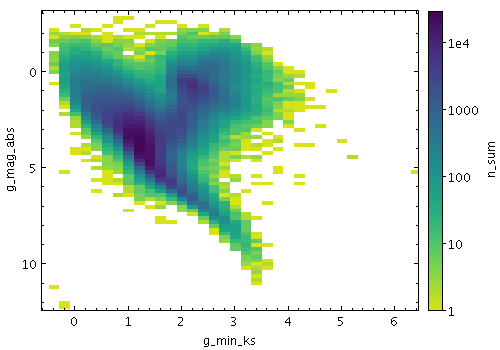
   stilts plot2plane layer1=grid in1=gk_hess.fits x1=g_min_ks y1=g_mag_abs
                     weight1=n combine1=sum xbinsize1=0.2 ybinsize1=0.2 xphase1=0.5 yphase1=0.5
                     yflip=true auxfunc=log auxmap=viridis
combineN = sum|sum-per-unit|count|... (Combiner)
weight coordinate
is left blank, a weighting of unity is assumed.
The available options are:
sum: the sum of all the combined values per binsum-per-unit: the sum of all the combined values per unit of bin sizecount: the number of non-blank values per bin (weight is ignored)count-per-unit: the number of non-blank values per unit of bin size (weight is ignored)mean: the mean of the combined valuesmedian: the medianq1: first quartileq3: third quartilemin: the minimum of all the combined valuesmax: the maximum of all the combined valuesstdev: the sample standard deviation of the combined valuesstdev_pop: the population standard deviation of the combined valueshit: 1 if any values present, NaN otherwise (weight is ignored)[Default: mean]
icmdN = <cmds> (ProcessingStep[])
inN.
The value of this parameter is one or more of the filter
commands described in Section 6.1.
If more than one is given, they must be separated by
semicolon characters (";").
This parameter can be repeated multiple times on the same
command line to build up a list of processing steps.
The sequence of commands given in this way
defines the processing pipeline which is performed on the table.
Commands may alternatively be supplied in an external file,
by using the indirection character '@'.
Thus a value of "@filename"
causes the file filename to be read for a list
of filter commands to execute. The commands in the file
may be separated by newline characters and/or semicolons,
and lines which are blank or which start with a
'#' character are ignored.
A backslash character '\' at the end of a line
joins it with the following line.
ifmtN = <in-format> (String)
inN.
The known formats are listed in Section 5.1.1.
This flag can be used if you know what format your
table is in.
If it has the special value
(auto) (the default),
then an attempt will be
made to detect the format of the table automatically.
This cannot always be done correctly however, in which case
the program will exit with an error explaining which
formats were attempted.
This parameter is ignored for scheme-specified tables.
[Default: (auto)]
inN = <table> (StarTable)
-",
meaning standard input.
In this case the input format must be given explicitly
using the ifmtN
parameter.
Note that not all formats can be streamed in this way.:<scheme-name>:<scheme-args>.<" character at the start,
or a "|" character at the end
("<syscmd" or
"syscmd|").
This executes the given pipeline and reads from its
standard output.
This will probably only work on unix-like systems.istreamN = true|false (Boolean)
inN parameter
will be read as a stream.
It is necessary to give the
ifmtN parameter
in this case.
Depending on the required operations and processing mode,
this may cause the read to fail (sometimes it is necessary
to read the table more than once).
It is not normally necessary to set this flag;
in most cases the data will be streamed automatically
if that is the best thing to do.
However it can sometimes result in less resource usage when
processing large files in certain formats (such as VOTable).
This parameter is ignored for scheme-specified tables.
[Default: false]
transparencyN = 0..1 (Double)
[Default: 0]
weightN = <num-expr> (String)
The value is a numeric algebraic expression based on column names as described in Section 10.
xbinsizeN = +<extent>|-<count> (BinSizer)
If the supplied value is a positive number it is interpreted as a fixed size in data coordinates (if the X axis is logarithmic, the value is a fixed factor). If it is a negative number, then it will be interpreted as the approximate number of bins to display across the plot in the X direction (though an attempt is made to use only round numbers for bin sizes).
When setting this value graphically, you can use either the slider to adjust the bin count or the numeric entry field to fix the bin size.
[Default: -30]
xphaseN = <number> (Double)
A value of 0 (or any integer) will result in a bin boundary at X=0 (linear X axis) or X=1 (logarithmic X axis). A fractional value will give a bin boundary at that value multiplied by the bin width.
[Default: 0]
ybinsizeN = +<extent>|-<count> (BinSizer)
If the supplied value is a positive number it is interpreted as a fixed size in data coordinates (if the Y axis is logarithmic, the value is a fixed factor). If it is a negative number, then it will be interpreted as the approximate number of bins to display across the plot in the Y direction (though an attempt is made to use only round numbers for bin sizes).
When setting this value graphically, you can use either the slider to adjust the bin count or the numeric entry field to fix the bin size.
[Default: -30]
yphaseN = <number> (Double)
A value of 0 (or any integer) will result in a bin boundary at X=0 (linear X axis) or X=1 (logarithmic X axis). A fractional value will give a bin boundary at that value multiplied by the bin width.
[Default: 0]
fill
If a two-dimensional dataset represents a single-valued function, this plotter will fill the area underneath the function's curve with a solid colour. Parts of the surface which would only be partially covered (because of rapid function variation within the width of a single pixel) are represented using appropriate alpha-blending. The filled area may alternatively be that above the curve or to its left or right.
One example of its use is to reconstruct the appearance of a histogram plot from a set of histogram bins. For X,Y data which is not single-valued, the result may not be very useful.
Usage Overview:
   layerN=fill colorN=<rrggbb>|red|blue|... transparencyN=0..1
               horizontalN=true|false positiveN=true|false <pos-coord-paramsN>
               inN=<table> ifmtN=<in-format> istreamN=true|false icmdN=<cmds>
All the parameters listed here
affect only the relevant layer,
identified by the suffix
N.
<pos-coord-paramsN>
give a position for each row of the input table.
Their form depends on the plot geometry,
i.e. which plotting command is used.
For a plane plot (plot2plane)
the parameters would be
xN and yN.
The coordinate parameter values are in all cases strings
interpreted as numeric expressions based on column names.
These can be column names, fixed values or algebraic
expressions as described in Section 10.
Example:
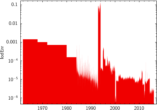
   stilts plot2time layer1=fill in1=iers.fits t1=decYear y1=lodErr yscale=log
                    texttype=latex fontsize=16
colorN = <rrggbb>|red|blue|... (Color)
The standard plotting colour names are
red, blue, green, grey, magenta, cyan, orange, pink, yellow, black, light_grey, white.
However, many other common colour names (too many to list here)
are also understood.
The list currently contains those colour names understood
by most web browsers,
from AliceBlue to YellowGreen,
listed e.g. in the
Extended color keywords section of
the CSS3 standard.
Alternatively, a six-digit hexadecimal number RRGGBB
may be supplied,
optionally prefixed by "#" or "0x",
giving red, green and blue intensities,
e.g. "ff00ff", "#ff00ff"
or "0xff00ff" for magenta.
[Default: red]
horizontalN = true|false (Boolean)
[Default: false]
icmdN = <cmds> (ProcessingStep[])
inN.
The value of this parameter is one or more of the filter
commands described in Section 6.1.
If more than one is given, they must be separated by
semicolon characters (";").
This parameter can be repeated multiple times on the same
command line to build up a list of processing steps.
The sequence of commands given in this way
defines the processing pipeline which is performed on the table.
Commands may alternatively be supplied in an external file,
by using the indirection character '@'.
Thus a value of "@filename"
causes the file filename to be read for a list
of filter commands to execute. The commands in the file
may be separated by newline characters and/or semicolons,
and lines which are blank or which start with a
'#' character are ignored.
A backslash character '\' at the end of a line
joins it with the following line.
ifmtN = <in-format> (String)
inN.
The known formats are listed in Section 5.1.1.
This flag can be used if you know what format your
table is in.
If it has the special value
(auto) (the default),
then an attempt will be
made to detect the format of the table automatically.
This cannot always be done correctly however, in which case
the program will exit with an error explaining which
formats were attempted.
This parameter is ignored for scheme-specified tables.
[Default: (auto)]
inN = <table> (StarTable)
-",
meaning standard input.
In this case the input format must be given explicitly
using the ifmtN
parameter.
Note that not all formats can be streamed in this way.:<scheme-name>:<scheme-args>.<" character at the start,
or a "|" character at the end
("<syscmd" or
"syscmd|").
This executes the given pipeline and reads from its
standard output.
This will probably only work on unix-like systems.istreamN = true|false (Boolean)
inN parameter
will be read as a stream.
It is necessary to give the
ifmtN parameter
in this case.
Depending on the required operations and processing mode,
this may cause the read to fail (sometimes it is necessary
to read the table more than once).
It is not normally necessary to set this flag;
in most cases the data will be streamed automatically
if that is the best thing to do.
However it can sometimes result in less resource usage when
processing large files in certain formats (such as VOTable).
This parameter is ignored for scheme-specified tables.
[Default: false]
positiveN = true|false (Boolean)
[Default: false]
transparencyN = 0..1 (Double)
[Default: 0]
vecfield
Plots a field of arrows on a regular grid corresponding to the aggregated (typically averaged) value of a 2-d vector quantity for the points in that grid cell.
Currently, the X and Y components of the vectors are
normalised separately and sized by default so that
the arrows are shown with components comparable to
the dimensions of the grid cells.
This length can be adjusted by use of the
scale option.
By default, the absolute values of the vectors are plotted.
However, if the
relative option
is set, the mean vector value averaged over the visible plot area
will be calculated and subtracted from all the plotted vectors.
The effect of this is to show local variations rather than
absolute values of the vectors over the visible area.
The X and Y dimensions of the grid cells (or equivalently histogram bins) can be configured either in terms of the data coordinates or relative to the plot dimensions.
Usage Overview:
   layerN=vecfield colorN=<rrggbb>|red|blue|...
                   arrowN=small_arrow|medium_arrow|... thickN=<int-value>
                   scaleN=<number> relativeN=true|false combineN=mean|sum
                   xbinsizeN=+<extent>|-<count> ybinsizeN=+<extent>|-<count>
                   xphaseN=<number> yphaseN=<number> xN=<num-expr>
                   yN=<num-expr> vxN=<num-expr> vyN=<num-expr>
                   weightN=<num-expr> inN=<table> ifmtN=<in-format>
                   istreamN=true|false icmdN=<cmds>
All the parameters listed here
affect only the relevant layer,
identified by the suffix
N.
Example:
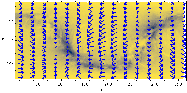
   stilts plot2plane xpix=600 ypix=300
                     in=tgas_source.fits x=ra y=dec
                     layer_1=mark shading_1=density densemap_1=cividis densefunc_1=linear
                     layer_2=vecfield vx_2=pmra vy_2=pmdec color_2=blue arrow_2=medium_arrow thick_2=1
arrowN = small_arrow|medium_arrow|... (MultiPointShape)
The available options are:
small_arrow
medium_arrow
large_arrow
small_open_dart
medium_open_dart
large_open_dart
small_filled_dart
medium_filled_dart
large_filled_dart
lines
capped_lines
[Default: small_arrow]
colorN = <rrggbb>|red|blue|... (Color)
The standard plotting colour names are
red, blue, green, grey, magenta, cyan, orange, pink, yellow, black, light_grey, white.
However, many other common colour names (too many to list here)
are also understood.
The list currently contains those colour names understood
by most web browsers,
from AliceBlue to YellowGreen,
listed e.g. in the
Extended color keywords section of
the CSS3 standard.
Alternatively, a six-digit hexadecimal number RRGGBB
may be supplied,
optionally prefixed by "#" or "0x",
giving red, green and blue intensities,
e.g. "ff00ff", "#ff00ff"
or "0xff00ff" for magenta.
[Default: red]
combineN = mean|sum (Combiner)
The available options are:
mean: the mean of the combined valuessum: the sum of all the combined values per bin[Default: mean]
icmdN = <cmds> (ProcessingStep[])
inN.
The value of this parameter is one or more of the filter
commands described in Section 6.1.
If more than one is given, they must be separated by
semicolon characters (";").
This parameter can be repeated multiple times on the same
command line to build up a list of processing steps.
The sequence of commands given in this way
defines the processing pipeline which is performed on the table.
Commands may alternatively be supplied in an external file,
by using the indirection character '@'.
Thus a value of "@filename"
causes the file filename to be read for a list
of filter commands to execute. The commands in the file
may be separated by newline characters and/or semicolons,
and lines which are blank or which start with a
'#' character are ignored.
A backslash character '\' at the end of a line
joins it with the following line.
ifmtN = <in-format> (String)
inN.
The known formats are listed in Section 5.1.1.
This flag can be used if you know what format your
table is in.
If it has the special value
(auto) (the default),
then an attempt will be
made to detect the format of the table automatically.
This cannot always be done correctly however, in which case
the program will exit with an error explaining which
formats were attempted.
This parameter is ignored for scheme-specified tables.
[Default: (auto)]
inN = <table> (StarTable)
-",
meaning standard input.
In this case the input format must be given explicitly
using the ifmtN
parameter.
Note that not all formats can be streamed in this way.:<scheme-name>:<scheme-args>.<" character at the start,
or a "|" character at the end
("<syscmd" or
"syscmd|").
This executes the given pipeline and reads from its
standard output.
This will probably only work on unix-like systems.istreamN = true|false (Boolean)
inN parameter
will be read as a stream.
It is necessary to give the
ifmtN parameter
in this case.
Depending on the required operations and processing mode,
this may cause the read to fail (sometimes it is necessary
to read the table more than once).
It is not normally necessary to set this flag;
in most cases the data will be streamed automatically
if that is the best thing to do.
However it can sometimes result in less resource usage when
processing large files in certain formats (such as VOTable).
This parameter is ignored for scheme-specified tables.
[Default: false]
relativeN = true|false (Boolean)
[Default: false]
scaleN = <number> (Double)
[Default: 1]
thickN = <int-value> (Integer)
[Default: 0]
vxN = <num-expr> (String)
The value is a numeric algebraic expression based on column names as described in Section 10.
vyN = <num-expr> (String)
The value is a numeric algebraic expression based on column names as described in Section 10.
weightN = <num-expr> (String)
The value is a numeric algebraic expression based on column names as described in Section 10.
xN = <num-expr> (String)
The value is a numeric algebraic expression based on column names as described in Section 10.
xbinsizeN = +<extent>|-<count> (BinSizer)
If the supplied value is a positive number it is interpreted as a fixed size in data coordinates (if the X axis is logarithmic, the value is a fixed factor). If it is a negative number, then it will be interpreted as the approximate number of bins to display across the plot in the X direction (though an attempt is made to use only round numbers for bin sizes).
When setting this value graphically, you can use either the slider to adjust the bin count or the numeric entry field to fix the bin size.
[Default: -16]
xphaseN = <number> (Double)
A value of 0 (or any integer) will result in a bin boundary at X=0 (linear X axis) or X=1 (logarithmic X axis). A fractional value will give a bin boundary at that value multiplied by the bin width.
[Default: 0]
yN = <num-expr> (String)
The value is a numeric algebraic expression based on column names as described in Section 10.
ybinsizeN = +<extent>|-<count> (BinSizer)
If the supplied value is a positive number it is interpreted as a fixed size in data coordinates (if the Y axis is logarithmic, the value is a fixed factor). If it is a negative number, then it will be interpreted as the approximate number of bins to display across the plot in the Y direction (though an attempt is made to use only round numbers for bin sizes).
When setting this value graphically, you can use either the slider to adjust the bin count or the numeric entry field to fix the bin size.
[Default: -16]
yphaseN = <number> (Double)
A value of 0 (or any integer) will result in a bin boundary at X=0 (linear X axis) or X=1 (logarithmic X axis). A fractional value will give a bin boundary at that value multiplied by the bin width.
[Default: 0]
quantile
Plots a line through a given quantile of the values binned within each pixel column (or row) of a plot. The line is optionally smoothed using a configurable kernel and width, to even out noise arising from the pixel binning. Instead of a simple line through a given quantile, it is also possible to fill the region between two quantiles.
One way to use this is to draw a line estimating a function y=f(x) (or x=g(y)) sampled by a noisy set of data points in two dimensions.
Note: in the current implementation, depending on the details of the configuration and the data, there may be some distortions or missing graphics near the edges of the plot. This may be improved in future releases, depending on feedback.
Usage Overview:
   layerN=quantile colorN=<rrggbb>|red|blue|... transparencyN=0..1
                   quantilesN=<low-frac>[,<high-frac>] thickN=<pixels>
                   smoothN=+<width>|-<count>
                   kernelN=square|linear|epanechnikov|cos|cos2|gauss3|gauss6
                   joinN=none|polygon|lines horizontalN=true|false
                   <pos-coord-paramsN> inN=<table> ifmtN=<in-format>
                   istreamN=true|false icmdN=<cmds>
All the parameters listed here
affect only the relevant layer,
identified by the suffix
N.
<pos-coord-paramsN>
give a position for each row of the input table.
Their form depends on the plot geometry,
i.e. which plotting command is used.
For a plane plot (plot2plane)
the parameters would be
xN and yN.
The coordinate parameter values are in all cases strings
interpreted as numeric expressions based on column names.
These can be column names, fixed values or algebraic
expressions as described in Section 10.
Example:
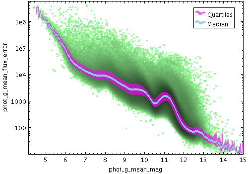
   stilts plot2plane in=tgas_source.fits x=phot_g_mean_mag y=phot_g_mean_flux_error
                     yscale=log xmax=15 ymin=10
                     layer.d=mark color.d=99ff99
                     layer.q4=quantile quantiles.q4=0.25,0.75 color.q4=magenta transparency.q4=0.35
                     layer.q2=quantile quantiles.q2=0.5 color.q2=SkyBlue thick.q2=4
                     smooth.q=0.05
                     leglabel.q4=Quartiles leglabel.q2=Median legseq=.q4,.q2 legpos=0.95,0.95
colorN = <rrggbb>|red|blue|... (Color)
The standard plotting colour names are
red, blue, green, grey, magenta, cyan, orange, pink, yellow, black, light_grey, white.
However, many other common colour names (too many to list here)
are also understood.
The list currently contains those colour names understood
by most web browsers,
from AliceBlue to YellowGreen,
listed e.g. in the
Extended color keywords section of
the CSS3 standard.
Alternatively, a six-digit hexadecimal number RRGGBB
may be supplied,
optionally prefixed by "#" or "0x",
giving red, green and blue intensities,
e.g. "ff00ff", "#ff00ff"
or "0xff00ff" for magenta.
[Default: red]
horizontalN = true|false (Boolean)
true, y quantiles are calculated
for each pixel column, and
if false, x quantiles are calculated
for each pixel row.
[Default: true]
icmdN = <cmds> (ProcessingStep[])
inN.
The value of this parameter is one or more of the filter
commands described in Section 6.1.
If more than one is given, they must be separated by
semicolon characters (";").
This parameter can be repeated multiple times on the same
command line to build up a list of processing steps.
The sequence of commands given in this way
defines the processing pipeline which is performed on the table.
Commands may alternatively be supplied in an external file,
by using the indirection character '@'.
Thus a value of "@filename"
causes the file filename to be read for a list
of filter commands to execute. The commands in the file
may be separated by newline characters and/or semicolons,
and lines which are blank or which start with a
'#' character are ignored.
A backslash character '\' at the end of a line
joins it with the following line.
ifmtN = <in-format> (String)
inN.
The known formats are listed in Section 5.1.1.
This flag can be used if you know what format your
table is in.
If it has the special value
(auto) (the default),
then an attempt will be
made to detect the format of the table automatically.
This cannot always be done correctly however, in which case
the program will exit with an error explaining which
formats were attempted.
This parameter is ignored for scheme-specified tables.
[Default: (auto)]
inN = <table> (StarTable)
-",
meaning standard input.
In this case the input format must be given explicitly
using the ifmtN
parameter.
Note that not all formats can be streamed in this way.:<scheme-name>:<scheme-args>.<" character at the start,
or a "|" character at the end
("<syscmd" or
"syscmd|").
This executes the given pipeline and reads from its
standard output.
This will probably only work on unix-like systems.istreamN = true|false (Boolean)
inN parameter
will be read as a stream.
It is necessary to give the
ifmtN parameter
in this case.
Depending on the required operations and processing mode,
this may cause the read to fail (sometimes it is necessary
to read the table more than once).
It is not normally necessary to set this flag;
in most cases the data will be streamed automatically
if that is the best thing to do.
However it can sometimes result in less resource usage when
processing large files in certain formats (such as VOTable).
This parameter is ignored for scheme-specified tables.
[Default: false]
joinN = none|polygon|lines (QJoin)
The available options are:
none: displayed quantile ranges are not joinedpolygon: the area between a line connecting the upper quantiles and a line connecting the lower quantiles is filledlines: a line of thickness given by thick is drawn from the center of each quantile range to the next[Default: none]
kernelN = square|linear|epanechnikov|cos|cos2|gauss3|gauss6 (Kernel1dShape)
The available options are:
square: Uniform value: f(x)=1, |x|=0..1linear: Triangle: f(x)=1-|x|, |x|=0..1epanechnikov: Parabola: f(x)=1-x*x, |x|=0..1cos: Cosine: f(x)=cos(x*pi/2), |x|=0..1cos2: Cosine squared: f(x)=cos^2(x*pi/2), |x|=0..1gauss3: Gaussian truncated at 3.0 sigma: f(x)=exp(-x*x/2), |x|=0..3gauss6: Gaussian truncated at 6.0 sigma: f(x)=exp(-x*x/2), |x|=0..6[Default: epanechnikov]
quantilesN = <low-frac>[,<high-frac>] (Subrange)
<lo>,<hi>)
indicating two quantile lines bounding an area to be filled.
A pair of equal values "a,a"
is equivalent to the single value "a".
The default is 0.5,
which means to mark the median value in each column,
and could equivalently be specified 0.5,0.5.
[Default: 0.5]
smoothN = +<width>|-<count> (BinSizer)
If the supplied value is a positive number it is interpreted as a fixed width in the data coordinates of the X axis (if the X axis is logarithmic, the value is a fixed factor). If it is a negative number, then it will be interpreted as the approximate number of smooothing widths that fit in the width of the visible plot (i.e. plot width / smoothing width). If the value is zero, no smoothing is applied.
When setting this value graphically, you can use either the slider to adjust the bin count or the numeric entry field to fix the bin width.
[Default: 0]
thickN = <pixels> (Integer)
quantiles
specifies a single value rather than a pair)
this will give the actual thickness of the plotted line.
If the range is non-zero however, the line may be thicker
than this in places according to the quantile positions.
[Default: 3]
transparencyN = 0..1 (Double)
[Default: 0]
histogram
Plots a histogram.
Bin heights may optionally be weighted by the
values of some additional coordinate,
supplied using the
weight
parameter.
In this case you can choose how these weights are combined
in each bin using the
combine
parameter.
Various options are provided for configuring how the bar heights are calculated, but note that not all combinations of the available parameters will necessarily lead to meaningful visualisations.
Usage Overview:
   layerN=histogram colorN=<rrggbb>|red|blue|... transparencyN=0..1
                    binsizeN=+<width>|-<count> phaseN=<number>
                    combineN=sum|sum-per-unit|count|... sidewaysN=true|false
                    cumulativeN=none|forward|reverse
                    normaliseN=none|area|unit|maximum|height
                    barformN=open|filled|semi_filled|steps|semi_steps|spikes
                    thickN=<pixels> dashN=dot|dash|...|<a,b,...> xN=<num-expr>
                    weightN=<num-expr> inN=<table> ifmtN=<in-format>
                    istreamN=true|false icmdN=<cmds>
All the parameters listed here
affect only the relevant layer,
identified by the suffix
N.
Example:
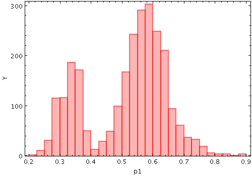
stilts plot2plane layer1=histogram in1=rrlyrae.fits x1=p1
barformN = open|filled|semi_filled|steps|semi_steps|spikes (Form)
The available options are:
open
filled
semi_filled
steps
semi_steps
spikes
[Default: semi_filled]
binsizeN = +<width>|-<count> (BinSizer)
When setting this value graphically, you can use either the slider to adjust the bin count or the numeric entry field to fix the bin width.
[Default: -30]
colorN = <rrggbb>|red|blue|... (Color)
The standard plotting colour names are
red, blue, green, grey, magenta, cyan, orange, pink, yellow, black, light_grey, white.
However, many other common colour names (too many to list here)
are also understood.
The list currently contains those colour names understood
by most web browsers,
from AliceBlue to YellowGreen,
listed e.g. in the
Extended color keywords section of
the CSS3 standard.
Alternatively, a six-digit hexadecimal number RRGGBB
may be supplied,
optionally prefixed by "#" or "0x",
giving red, green and blue intensities,
e.g. "ff00ff", "#ff00ff"
or "0xff00ff" for magenta.
[Default: red]
combineN = sum|sum-per-unit|count|... (Combiner)
weight coordinate,
but if no weight is supplied,
a weighting of unity is assumed.
The available options are:
sum: the sum of all the combined values per binsum-per-unit: the sum of all the combined values per unit of bin sizecount: the number of non-blank values per bin (weight is ignored)count-per-unit: the number of non-blank values per unit of bin size (weight is ignored)mean: the mean of the combined valuesmedian: the medianq1: first quartileq3: third quartilemin: the minimum of all the combined valuesmax: the maximum of all the combined valuesstdev: the sample standard deviation of the combined valuesstdev_pop: the population standard deviation of the combined valueshit: 1 if any values present, NaN otherwise (weight is ignored)[Default: sum]
cumulativeN = none|forward|reverse (Cumulation)
forward/reverse
the histogram bars plotted are calculated
cumulatively;
each bin includes the counts from all previous bins
working up/down the independent axis.
Note that setting cumulative plotting may not make much sense with some other parameter values, for instance averaging aggregation modes.
For reasons of backward compatibility,
the values true and false
may be used as aliases for
forward and none.
The available options are:
none: The value plotted for each bin uses the samples accumulated in that bin.forward: The value plotted for each bin uses the samples accumulated all the way from negative infinity to that bin.reverse: The value plotted for each bin uses the samples accumulated all the way from positive infinity to that bin.[Default: none]
dashN = dot|dash|...|<a,b,...> (float[])
Possible values for dashed lines are
dot, dash, longdash, dotdash.
You can alternatively supply a comma-separated list
of on/off length values such as
"4,2,8,2".
icmdN = <cmds> (ProcessingStep[])
inN.
The value of this parameter is one or more of the filter
commands described in Section 6.1.
If more than one is given, they must be separated by
semicolon characters (";").
This parameter can be repeated multiple times on the same
command line to build up a list of processing steps.
The sequence of commands given in this way
defines the processing pipeline which is performed on the table.
Commands may alternatively be supplied in an external file,
by using the indirection character '@'.
Thus a value of "@filename"
causes the file filename to be read for a list
of filter commands to execute. The commands in the file
may be separated by newline characters and/or semicolons,
and lines which are blank or which start with a
'#' character are ignored.
A backslash character '\' at the end of a line
joins it with the following line.
ifmtN = <in-format> (String)
inN.
The known formats are listed in Section 5.1.1.
This flag can be used if you know what format your
table is in.
If it has the special value
(auto) (the default),
then an attempt will be
made to detect the format of the table automatically.
This cannot always be done correctly however, in which case
the program will exit with an error explaining which
formats were attempted.
This parameter is ignored for scheme-specified tables.
[Default: (auto)]
inN = <table> (StarTable)
-",
meaning standard input.
In this case the input format must be given explicitly
using the ifmtN
parameter.
Note that not all formats can be streamed in this way.:<scheme-name>:<scheme-args>.<" character at the start,
or a "|" character at the end
("<syscmd" or
"syscmd|").
This executes the given pipeline and reads from its
standard output.
This will probably only work on unix-like systems.istreamN = true|false (Boolean)
inN parameter
will be read as a stream.
It is necessary to give the
ifmtN parameter
in this case.
Depending on the required operations and processing mode,
this may cause the read to fail (sometimes it is necessary
to read the table more than once).
It is not normally necessary to set this flag;
in most cases the data will be streamed automatically
if that is the best thing to do.
However it can sometimes result in less resource usage when
processing large files in certain formats (such as VOTable).
This parameter is ignored for scheme-specified tables.
[Default: false]
normaliseN = none|area|unit|maximum|height (Normalisation)
Note that some of the normalisation options may not make much sense with some other parameter values, for instance averaging aggregation modes.
The available options are:
none: No normalisation is performed.area: The total area of histogram bars is normalised to unity. For cumulative plots, this behaves like height.unit: Histogram bars are scaled by the inverse of the bin width in data units. For cumulative plots, this behaves like none.maximum: The height of the tallest histogram bar is normalised to unity. For cumulative plots, this behaves like height.height: The total height of histogram bars is normalised to unity.[Default: none]
phaseN = <number> (Double)
A value of 0 (or any integer) will result in a bin boundary at X=0 (linear X axis) or X=1 (logarithmic X axis). A fractional value will give a bin boundary at that value multiplied by the bin width.
[Default: 0]
sidewaysN = true|false (Boolean)
false,
the quantity being accumulated is on the the horizontal axis
and the frequency is represented vertically as usual.
If set true the quantity accumulated
is on the vertical axis,
and the frequency is represented horizontally,
so that the chart is displayed reflected in the X=Y line.
[Default: false]
thickN = <pixels> (Integer)
[Default: 2]
transparencyN = 0..1 (Double)
[Default: 0]
weightN = <num-expr> (String)
The value is a numeric algebraic expression based on column names as described in Section 10.
xN = <num-expr> (String)
The value is a numeric algebraic expression based on column names as described in Section 10.
kde
Plots a Discrete Kernel Density Estimate giving a smoothed frequency of data values along the horizontal axis, using a fixed-width smoothing kernel. This is a generalisation of a histogram in which the bins are always 1 pixel wide, and a smoothing kernel is applied to each bin. The width and shape of the kernel may be varied.
This is suitable for cases where the division into discrete bins done by a normal histogram is unnecessary or troublesome.
Note this is not a true Kernel Density Estimate, since, for performance reasons, the smoothing is applied to the (pixel-width) bins rather than to each data sample. The deviation from a true KDE caused by this quantisation will be at the pixel level, hence in most cases not visually apparent.
A weighting may be applied to the calculated levels
by supplying the
weight
coordinate.
In this case you can choose how these weights are aggregated
in each pixel bin using the
combine
parameter.
The result is something like a smoothed version of the
corresponding weighted histogram.
Note that some combinations of the available parameters
(e.g. a normalised cumulative median-aggregated KDE)
may not make much visual sense.
Usage Overview:
   layerN=kde colorN=<rrggbb>|red|blue|... transparencyN=0..1
              sidewaysN=true|false smoothN=+<width>|-<count>
              combineN=sum|sum-per-unit|count|...
              kernelN=square|linear|epanechnikov|cos|cos2|gauss3|gauss6
              cumulativeN=none|forward|reverse
              normaliseN=none|area|unit|maximum|height fillN=solid|line|semi
              thickN=<pixels> xN=<num-expr> weightN=<num-expr> inN=<table>
              ifmtN=<in-format> istreamN=true|false icmdN=<cmds>
All the parameters listed here
affect only the relevant layer,
identified by the suffix
N.
Example:
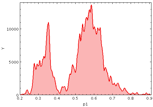
stilts plot2plane ymin=0 layer1=kde in1=rrlyrae.fits x1=p1
colorN = <rrggbb>|red|blue|... (Color)
The standard plotting colour names are
red, blue, green, grey, magenta, cyan, orange, pink, yellow, black, light_grey, white.
However, many other common colour names (too many to list here)
are also understood.
The list currently contains those colour names understood
by most web browsers,
from AliceBlue to YellowGreen,
listed e.g. in the
Extended color keywords section of
the CSS3 standard.
Alternatively, a six-digit hexadecimal number RRGGBB
may be supplied,
optionally prefixed by "#" or "0x",
giving red, green and blue intensities,
e.g. "ff00ff", "#ff00ff"
or "0xff00ff" for magenta.
[Default: red]
combineN = sum|sum-per-unit|count|... (Combiner)
sum-per-unit and
mean make sense,
others such as
sum do not.
The combined values are those given by the
weight coordinate,
but if no weight is supplied,
a weighting of unity is assumed.
The available options are:
sum: the sum of all the combined values per binsum-per-unit: the sum of all the combined values per unit of bin sizecount: the number of non-blank values per bin (weight is ignored)count-per-unit: the number of non-blank values per unit of bin size (weight is ignored)mean: the mean of the combined valuesmedian: the medianq1: first quartileq3: third quartilemin: the minimum of all the combined valuesmax: the maximum of all the combined valuesstdev: the sample standard deviation of the combined valuesstdev_pop: the population standard deviation of the combined valueshit: 1 if any values present, NaN otherwise (weight is ignored)[Default: sum-per-unit]
cumulativeN = none|forward|reverse (Cumulation)
forward/reverse
the histogram bars plotted are calculated
cumulatively;
each bin includes the counts from all previous bins
working up/down the independent axis.
Note that setting cumulative plotting may not make much sense with some other parameter values, for instance averaging aggregation modes.
For reasons of backward compatibility,
the values true and false
may be used as aliases for
forward and none.
The available options are:
none: The value plotted for each bin uses the samples accumulated in that bin.forward: The value plotted for each bin uses the samples accumulated all the way from negative infinity to that bin.reverse: The value plotted for each bin uses the samples accumulated all the way from positive infinity to that bin.[Default: none]
fillN = solid|line|semi (FillMode)
The available options are:
solid: area between level and axis is filled with solid colourline: level is marked by a wiggly linesemi: level is marked by a wiggly line, and area below it is filled with a transparent colour[Default: semi]
icmdN = <cmds> (ProcessingStep[])
inN.
The value of this parameter is one or more of the filter
commands described in Section 6.1.
If more than one is given, they must be separated by
semicolon characters (";").
This parameter can be repeated multiple times on the same
command line to build up a list of processing steps.
The sequence of commands given in this way
defines the processing pipeline which is performed on the table.
Commands may alternatively be supplied in an external file,
by using the indirection character '@'.
Thus a value of "@filename"
causes the file filename to be read for a list
of filter commands to execute. The commands in the file
may be separated by newline characters and/or semicolons,
and lines which are blank or which start with a
'#' character are ignored.
A backslash character '\' at the end of a line
joins it with the following line.
ifmtN = <in-format> (String)
inN.
The known formats are listed in Section 5.1.1.
This flag can be used if you know what format your
table is in.
If it has the special value
(auto) (the default),
then an attempt will be
made to detect the format of the table automatically.
This cannot always be done correctly however, in which case
the program will exit with an error explaining which
formats were attempted.
This parameter is ignored for scheme-specified tables.
[Default: (auto)]
inN = <table> (StarTable)
-",
meaning standard input.
In this case the input format must be given explicitly
using the ifmtN
parameter.
Note that not all formats can be streamed in this way.:<scheme-name>:<scheme-args>.<" character at the start,
or a "|" character at the end
("<syscmd" or
"syscmd|").
This executes the given pipeline and reads from its
standard output.
This will probably only work on unix-like systems.istreamN = true|false (Boolean)
inN parameter
will be read as a stream.
It is necessary to give the
ifmtN parameter
in this case.
Depending on the required operations and processing mode,
this may cause the read to fail (sometimes it is necessary
to read the table more than once).
It is not normally necessary to set this flag;
in most cases the data will be streamed automatically
if that is the best thing to do.
However it can sometimes result in less resource usage when
processing large files in certain formats (such as VOTable).
This parameter is ignored for scheme-specified tables.
[Default: false]
kernelN = square|linear|epanechnikov|cos|cos2|gauss3|gauss6 (Kernel1dShape)
The available options are:
square: Uniform value: f(x)=1, |x|=0..1linear: Triangle: f(x)=1-|x|, |x|=0..1epanechnikov: Parabola: f(x)=1-x*x, |x|=0..1cos: Cosine: f(x)=cos(x*pi/2), |x|=0..1cos2: Cosine squared: f(x)=cos^2(x*pi/2), |x|=0..1gauss3: Gaussian truncated at 3.0 sigma: f(x)=exp(-x*x/2), |x|=0..3gauss6: Gaussian truncated at 6.0 sigma: f(x)=exp(-x*x/2), |x|=0..6[Default: epanechnikov]
normaliseN = none|area|unit|maximum|height (Normalisation)
Note that some of the normalisation options may not make much sense with some other parameter values, for instance averaging aggregation modes.
The available options are:
none: No normalisation is performed.area: The total area of histogram bars is normalised to unity. For cumulative plots, this behaves like height.unit: Histogram bars are scaled by the inverse of the bin width in data units. For cumulative plots, this behaves like none.maximum: The height of the tallest histogram bar is normalised to unity. For cumulative plots, this behaves like height.height: The total height of histogram bars is normalised to unity.[Default: none]
sidewaysN = true|false (Boolean)
false,
the quantity being accumulated is on the the horizontal axis
and the frequency is represented vertically as usual.
If set true the quantity accumulated
is on the vertical axis,
and the frequency is represented horizontally,
so that the chart is displayed reflected in the X=Y line.
[Default: false]
smoothN = +<width>|-<count> (BinSizer)
If the supplied value is a positive number it is interpreted as a fixed width in the data coordinates of the X axis (if the X axis is logarithmic, the value is a fixed factor). If it is a negative number, then it will be interpreted as the approximate number of smooothing widths that fit in the width of the visible plot (i.e. plot width / smoothing width). If the value is zero, no smoothing is applied.
When setting this value graphically, you can use either the slider to adjust the bin count or the numeric entry field to fix the bin width.
[Default: -100]
thickN = <pixels> (Integer)
[Default: 2]
transparencyN = 0..1 (Double)
[Default: 0]
weightN = <num-expr> (String)
The value is a numeric algebraic expression based on column names as described in Section 10.
xN = <num-expr> (String)
The value is a numeric algebraic expression based on column names as described in Section 10.
knn
Plots a Discrete Kernel Density Estimate giving a smoothed frequency of data values along the horizontal axis, using an adaptive (K-Nearest-Neighbours) smoothing kernel. This is a generalisation of a histogram in which the bins are always 1 pixel wide, and a smoothing kernel is applied to each bin. The width and shape of the kernel may be varied.
The K-Nearest-Neighbour figure gives the number of points in each direction to determine the width of the smoothing kernel for smoothing each bin. Upper and lower limits for the kernel width are also supplied; if the upper and lower limits are equal, this is equivalent to a fixed-width kernel.
Note this is not a true Kernel Density Estimate, since, for performance reasons, the smoothing is applied to the (pixel-width) bins rather than to each data sample. The deviation from a true KDE caused by this quantisation will be at the pixel level, hence in most cases not visually apparent.
Usage Overview:
   layerN=knn colorN=<rrggbb>|red|blue|... transparencyN=0..1
              sidewaysN=true|false knnN=<number> symmetricN=true|false
              minsmoothN=+<width>|-<count> maxsmoothN=+<width>|-<count>
              kernelN=square|linear|epanechnikov|cos|cos2|gauss3|gauss6
              cumulativeN=none|forward|reverse
              normaliseN=none|area|unit|maximum|height fillN=solid|line|semi
              thickN=<pixels> xN=<num-expr> weightN=<num-expr> inN=<table>
              ifmtN=<in-format> istreamN=true|false icmdN=<cmds>
All the parameters listed here
affect only the relevant layer,
identified by the suffix
N.
Example:
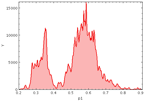
stilts plot2plane layer1=knn in1=rrlyrae.fits x1=p1
colorN = <rrggbb>|red|blue|... (Color)
The standard plotting colour names are
red, blue, green, grey, magenta, cyan, orange, pink, yellow, black, light_grey, white.
However, many other common colour names (too many to list here)
are also understood.
The list currently contains those colour names understood
by most web browsers,
from AliceBlue to YellowGreen,
listed e.g. in the
Extended color keywords section of
the CSS3 standard.
Alternatively, a six-digit hexadecimal number RRGGBB
may be supplied,
optionally prefixed by "#" or "0x",
giving red, green and blue intensities,
e.g. "ff00ff", "#ff00ff"
or "0xff00ff" for magenta.
[Default: red]
cumulativeN = none|forward|reverse (Cumulation)
forward/reverse
the histogram bars plotted are calculated
cumulatively;
each bin includes the counts from all previous bins
working up/down the independent axis.
Note that setting cumulative plotting may not make much sense with some other parameter values, for instance averaging aggregation modes.
For reasons of backward compatibility,
the values true and false
may be used as aliases for
forward and none.
The available options are:
none: The value plotted for each bin uses the samples accumulated in that bin.forward: The value plotted for each bin uses the samples accumulated all the way from negative infinity to that bin.reverse: The value plotted for each bin uses the samples accumulated all the way from positive infinity to that bin.[Default: none]
fillN = solid|line|semi (FillMode)
The available options are:
solid: area between level and axis is filled with solid colourline: level is marked by a wiggly linesemi: level is marked by a wiggly line, and area below it is filled with a transparent colour[Default: semi]
icmdN = <cmds> (ProcessingStep[])
inN.
The value of this parameter is one or more of the filter
commands described in Section 6.1.
If more than one is given, they must be separated by
semicolon characters (";").
This parameter can be repeated multiple times on the same
command line to build up a list of processing steps.
The sequence of commands given in this way
defines the processing pipeline which is performed on the table.
Commands may alternatively be supplied in an external file,
by using the indirection character '@'.
Thus a value of "@filename"
causes the file filename to be read for a list
of filter commands to execute. The commands in the file
may be separated by newline characters and/or semicolons,
and lines which are blank or which start with a
'#' character are ignored.
A backslash character '\' at the end of a line
joins it with the following line.
ifmtN = <in-format> (String)
inN.
The known formats are listed in Section 5.1.1.
This flag can be used if you know what format your
table is in.
If it has the special value
(auto) (the default),
then an attempt will be
made to detect the format of the table automatically.
This cannot always be done correctly however, in which case
the program will exit with an error explaining which
formats were attempted.
This parameter is ignored for scheme-specified tables.
[Default: (auto)]
inN = <table> (StarTable)
-",
meaning standard input.
In this case the input format must be given explicitly
using the ifmtN
parameter.
Note that not all formats can be streamed in this way.:<scheme-name>:<scheme-args>.<" character at the start,
or a "|" character at the end
("<syscmd" or
"syscmd|").
This executes the given pipeline and reads from its
standard output.
This will probably only work on unix-like systems.istreamN = true|false (Boolean)
inN parameter
will be read as a stream.
It is necessary to give the
ifmtN parameter
in this case.
Depending on the required operations and processing mode,
this may cause the read to fail (sometimes it is necessary
to read the table more than once).
It is not normally necessary to set this flag;
in most cases the data will be streamed automatically
if that is the best thing to do.
However it can sometimes result in less resource usage when
processing large files in certain formats (such as VOTable).
This parameter is ignored for scheme-specified tables.
[Default: false]
kernelN = square|linear|epanechnikov|cos|cos2|gauss3|gauss6 (Kernel1dShape)
The available options are:
square: Uniform value: f(x)=1, |x|=0..1linear: Triangle: f(x)=1-|x|, |x|=0..1epanechnikov: Parabola: f(x)=1-x*x, |x|=0..1cos: Cosine: f(x)=cos(x*pi/2), |x|=0..1cos2: Cosine squared: f(x)=cos^2(x*pi/2), |x|=0..1gauss3: Gaussian truncated at 3.0 sigma: f(x)=exp(-x*x/2), |x|=0..3gauss6: Gaussian truncated at 6.0 sigma: f(x)=exp(-x*x/2), |x|=0..6[Default: epanechnikov]
knnN = <number> (Double)
The threshold is actually the weighted total of samples;
for unweighted (weight=1) bins
that is equivalent to the number of samples.
[Default: 100]
maxsmoothN = +<width>|-<count> (BinSizer)
If the supplied value is a positive number it is interpreted as a fixed width in the data coordinates of the X axis (if the X axis is logarithmic, the value is a fixed factor). If it is a negative number, then it will be interpreted as the approximate number of smooothing widths that fit in the width of the visible plot (i.e. plot width / smoothing width). If the value is zero, no smoothing is applied.
When setting this value graphically, you can use either the slider to adjust the bin count or the numeric entry field to fix the bin width.
[Default: -100]
minsmoothN = +<width>|-<count> (BinSizer)
If the supplied value is a positive number it is interpreted as a fixed width in the data coordinates of the X axis (if the X axis is logarithmic, the value is a fixed factor). If it is a negative number, then it will be interpreted as the approximate number of smooothing widths that fit in the width of the visible plot (i.e. plot width / smoothing width). If the value is zero, no smoothing is applied.
When setting this value graphically, you can use either the slider to adjust the bin count or the numeric entry field to fix the bin width.
[Default: 0]
normaliseN = none|area|unit|maximum|height (Normalisation)
Note that some of the normalisation options may not make much sense with some other parameter values, for instance averaging aggregation modes.
The available options are:
none: No normalisation is performed.area: The total area of histogram bars is normalised to unity. For cumulative plots, this behaves like height.unit: Histogram bars are scaled by the inverse of the bin width in data units. For cumulative plots, this behaves like none.maximum: The height of the tallest histogram bar is normalised to unity. For cumulative plots, this behaves like height.height: The total height of histogram bars is normalised to unity.[Default: none]
sidewaysN = true|false (Boolean)
false,
the quantity being accumulated is on the the horizontal axis
and the frequency is represented vertically as usual.
If set true the quantity accumulated
is on the vertical axis,
and the frequency is represented horizontally,
so that the chart is displayed reflected in the X=Y line.
[Default: false]
symmetricN = true|false (Boolean)
[Default: true]
thickN = <pixels> (Integer)
[Default: 2]
transparencyN = 0..1 (Double)
[Default: 0]
weightN = <num-expr> (String)
The value is a numeric algebraic expression based on column names as described in Section 10.
xN = <num-expr> (String)
The value is a numeric algebraic expression based on column names as described in Section 10.
densogram
Represents smoothed density of data values along the horizontal axis using a colourmap. This is like a Kernel Density Estimate (smoothed histogram with bins 1 pixel wide), but instead of representing the data extent vertically as bars or a line, values are represented by a fixed-size pixel-width column of a colour from a colour map. A smoothing kernel, whose width and shape may be varied, is applied to each data point.
A weighting may be applied to the calculated levels
by supplying the
weight
coordinate.
In this case you can choose how these weights are aggregated
in each pixel bin using the
combine
parameter.
The result is something like a smoothed version of the
corresponding weighted histogram.
Note that some combinations of the available parameters
(e.g. a normalised cumulative median-aggregated KDE)
may not make much visual sense.
This is a rather unconventional way to represent density data, and this plotting mode is probably not very useful. But hey, nobody's forcing you to use it.
Usage Overview:
   layerN=densogram colorN=<rrggbb>|red|blue|... smoothN=+<width>|-<count>
                    sidewaysN=true|false
                    kernelN=square|linear|epanechnikov|cos|cos2|gauss3|gauss6
                    densemapN=<map-name>|<color>-<color>[-<color>...]
                    denseclipN=<lo>,<hi> denseflipN=true|false
                    densequantN=<number> densesubN=<lo>,<hi>
                    densefuncN=log|linear|histogram|...
                    cumulativeN=none|forward|reverse sizeN=<pixels>
                    posN=<fraction> xN=<num-expr> weightN=<num-expr>
                    inN=<table> ifmtN=<in-format> istreamN=true|false
                    icmdN=<cmds>
All the parameters listed here
affect only the relevant layer,
identified by the suffix
N.
Example:
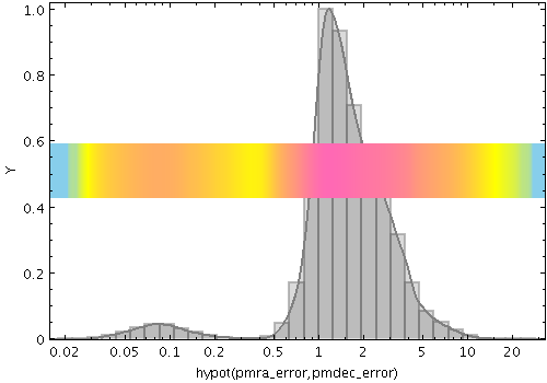
   stilts plot2plane in=tgas_source.fits x=hypot(pmra_error,pmdec_error)
                     xscale=log normalise=maximum
                     color=grey layer1=histogram layer2=kde
                     layer3=densogram densemap3=skyblue-yellow-hotpink densefunc3=log
                     size3=50 pos3=0.5
colorN = <rrggbb>|red|blue|... (Color)
The standard plotting colour names are
red, blue, green, grey, magenta, cyan, orange, pink, yellow, black, light_grey, white.
However, many other common colour names (too many to list here)
are also understood.
The list currently contains those colour names understood
by most web browsers,
from AliceBlue to YellowGreen,
listed e.g. in the
Extended color keywords section of
the CSS3 standard.
Alternatively, a six-digit hexadecimal number RRGGBB
may be supplied,
optionally prefixed by "#" or "0x",
giving red, green and blue intensities,
e.g. "ff00ff", "#ff00ff"
or "0xff00ff" for magenta.
[Default: red]
cumulativeN = none|forward|reverse (Cumulation)
forward/reverse
the histogram bars plotted are calculated
cumulatively;
each bin includes the counts from all previous bins
working up/down the independent axis.
Note that setting cumulative plotting may not make much sense with some other parameter values, for instance averaging aggregation modes.
For reasons of backward compatibility,
the values true and false
may be used as aliases for
forward and none.
The available options are:
none: The value plotted for each bin uses the samples accumulated in that bin.forward: The value plotted for each bin uses the samples accumulated all the way from negative infinity to that bin.reverse: The value plotted for each bin uses the samples accumulated all the way from positive infinity to that bin.[Default: none]
denseclipN = <lo>,<hi> (Subrange)
If the full range 0,1 is used,
the whole range of colours specified by the selected
shader will be used.
But if for instance a value of 0,0.5 is given,
only those colours at the left hand end of the ramp
will be seen.
If the null (default) value is chosen,
a default clip will be used.
This generally covers most or all of the range 0-1
but for colour maps which fade to white,
a small proportion of the lower end may be excluded,
to ensure that all the colours are visually distinguishable
from a white background.
This default is usually a good idea if the colour map
is being used with something like a scatter plot,
where markers are plotted against a white background.
However, for something like a density map when the whole
plotting area is tiled with colours from the map,
it may be better to supply the whole range
0,1 explicitly.
denseflipN = true|false (Boolean)
[Default: false]
densefuncN = log|linear|histogram|... (Scaling)
The available options are:
log: Logarithmic scaling, positive values onlylinear: Linear scalinghistogram: Scaling follows data distribution, with linear axishistolog: Scaling follows data distribution, with logarithmic axis, positive values onlyasinh: Asinh scaling, wide dynamic range for both positive and negative valuessqrt: Square root scalingsquare: Square scalingacos: Inverse cosine Scalingcos: Cosine ScalingFor all these options,
the full range of valid data values is used,
and displayed on the colour bar
if applicable (though it can be restricted using the densesub option)
Note that logarithmic-based options
Log and
HistoLog
will ignore non-positive values.
The Linear,
Log,
Square and
Sqrt options
just apply the named function to the full data range.
The histogram options on the other hand use a scaling function
that corresponds to the actual distribution of the data, so that
there are about the same number of points (or pixels, or whatever
is being scaled) of each colour.
The histogram options are somewhat more expensive,
but can be a good choice if you are exploring data whose
distribution is unknown or not well-behaved over
its min-max range.
The Histogram and
HistoLog options both
assign the colours in the same way, but they display the colour
ramp with linear or logarithmic annotation respectively;
the HistoLog option also ignores
non-positive values.
[Default: linear]
densemapN = <map-name>|<color>-<color>[-<color>...] (Shader)
A mixed bag of colour ramps are available
as listed in Section 8.7:
inferno,
magma,
plasma,
viridis,
cividis,
cubehelix,
sron,
rainbow,
rainbow2,
rainbow3,
pastel,
cosmic,
ember,
gothic,
rainforest,
voltage,
bubblegum,
gem,
chroma,
sunset,
neon,
tropical,
accent,
gnuplot,
gnuplot2,
specxby,
set1,
paired,
hotcold,
guppy,
iceburn,
redshift,
pride,
rdbu,
piyg,
brbg,
cyan-magenta,
red-blue,
brg,
heat,
cold,
light,
greyscale,
colour,
standard,
bugn,
bupu,
orrd,
pubu,
purd,
painbow,
huecl,
infinity,
hue,
intensity,
rgb_red,
rgb_green,
rgb_blue,
hsv_h,
hsv_s,
hsv_v,
yuv_y,
yuv_u,
yuv_v,
scale_hsv_s,
scale_hsv_v,
scale_yuv_y,
mask,
blacker,
whiter,
transparency.
Note:
many of these, including rainbow-like ones,
are frowned upon by the visualisation community.
You can also construct your own custom colour map
by giving a sequence of colour names separated by
minus sign ("-") characters.
In this case the ramp is a linear interpolation
between each pair of colours named,
using the same syntax as when specifying
a colour value.
So for instance
"yellow-hotpink-#0000ff"
would shade from yellow via hot pink to blue.
[Default: inferno]
densequantN = <number> (Double)
If left blank, the colour map is nominally continuous (though in practice it may be quantised to a medium-sized number like 256).
densesubN = <lo>,<hi> (Subrange)
The default value "0,1" therefore has
no effect.
The range could be restricted to its lower half
with the value 0,0.5.
[Default: 0,1]
icmdN = <cmds> (ProcessingStep[])
inN.
The value of this parameter is one or more of the filter
commands described in Section 6.1.
If more than one is given, they must be separated by
semicolon characters (";").
This parameter can be repeated multiple times on the same
command line to build up a list of processing steps.
The sequence of commands given in this way
defines the processing pipeline which is performed on the table.
Commands may alternatively be supplied in an external file,
by using the indirection character '@'.
Thus a value of "@filename"
causes the file filename to be read for a list
of filter commands to execute. The commands in the file
may be separated by newline characters and/or semicolons,
and lines which are blank or which start with a
'#' character are ignored.
A backslash character '\' at the end of a line
joins it with the following line.
ifmtN = <in-format> (String)
inN.
The known formats are listed in Section 5.1.1.
This flag can be used if you know what format your
table is in.
If it has the special value
(auto) (the default),
then an attempt will be
made to detect the format of the table automatically.
This cannot always be done correctly however, in which case
the program will exit with an error explaining which
formats were attempted.
This parameter is ignored for scheme-specified tables.
[Default: (auto)]
inN = <table> (StarTable)
-",
meaning standard input.
In this case the input format must be given explicitly
using the ifmtN
parameter.
Note that not all formats can be streamed in this way.:<scheme-name>:<scheme-args>.<" character at the start,
or a "|" character at the end
("<syscmd" or
"syscmd|").
This executes the given pipeline and reads from its
standard output.
This will probably only work on unix-like systems.istreamN = true|false (Boolean)
inN parameter
will be read as a stream.
It is necessary to give the
ifmtN parameter
in this case.
Depending on the required operations and processing mode,
this may cause the read to fail (sometimes it is necessary
to read the table more than once).
It is not normally necessary to set this flag;
in most cases the data will be streamed automatically
if that is the best thing to do.
However it can sometimes result in less resource usage when
processing large files in certain formats (such as VOTable).
This parameter is ignored for scheme-specified tables.
[Default: false]
kernelN = square|linear|epanechnikov|cos|cos2|gauss3|gauss6 (Kernel1dShape)
The available options are:
square: Uniform value: f(x)=1, |x|=0..1linear: Triangle: f(x)=1-|x|, |x|=0..1epanechnikov: Parabola: f(x)=1-x*x, |x|=0..1cos: Cosine: f(x)=cos(x*pi/2), |x|=0..1cos2: Cosine squared: f(x)=cos^2(x*pi/2), |x|=0..1gauss3: Gaussian truncated at 3.0 sigma: f(x)=exp(-x*x/2), |x|=0..3gauss6: Gaussian truncated at 6.0 sigma: f(x)=exp(-x*x/2), |x|=0..6[Default: epanechnikov]
posN = <fraction> (Double)
[Default: 0.05]
sidewaysN = true|false (Boolean)
false,
the quantity being accumulated is on the the horizontal axis
and the frequency is represented vertically as usual.
If set true the quantity accumulated
is on the vertical axis,
and the frequency is represented horizontally,
so that the chart is displayed reflected in the X=Y line.
[Default: false]
sizeN = <pixels> (Integer)
[Default: 12]
smoothN = +<width>|-<count> (BinSizer)
If the supplied value is a positive number it is interpreted as a fixed width in the data coordinates of the X axis (if the X axis is logarithmic, the value is a fixed factor). If it is a negative number, then it will be interpreted as the approximate number of smooothing widths that fit in the width of the visible plot (i.e. plot width / smoothing width). If the value is zero, no smoothing is applied.
When setting this value graphically, you can use either the slider to adjust the bin count or the numeric entry field to fix the bin width.
[Default: -100]
weightN = <num-expr> (String)
The value is a numeric algebraic expression based on column names as described in Section 10.
xN = <num-expr> (String)
The value is a numeric algebraic expression based on column names as described in Section 10.
gaussian
Plots a best fit Gaussian to the histogram of a sample of data. In fact, all this plotter does is to calculate the mean and standard deviation of the sample, and plot the corresponding Gaussian curve. The mean and standard deviation values are reported by the plot.
The normalise config option,
perhaps in conjunction with binsize,
can be used to scale the height of the plotted curve
in data units.
In this case, binsize
just describes the bar width of a notional histogram
whose outline the plotted Gaussian should try to fit,
and is only relevant for some of the normalisation options.
Usage Overview:
   layerN=gaussian colorN=<rrggbb>|red|blue|... showmeanN=true|false
                   sidewaysN=true|false thickN=<pixels>
                   dashN=dot|dash|...|<a,b,...> antialiasN=true|false
                   normaliseN=none|area|unit|maximum|height
                   binsizeN=+<width>|-<count> xN=<num-expr> weightN=<num-expr>
                   inN=<table> ifmtN=<in-format> istreamN=true|false
                   icmdN=<cmds>
All the parameters listed here
affect only the relevant layer,
identified by the suffix
N.
Example:
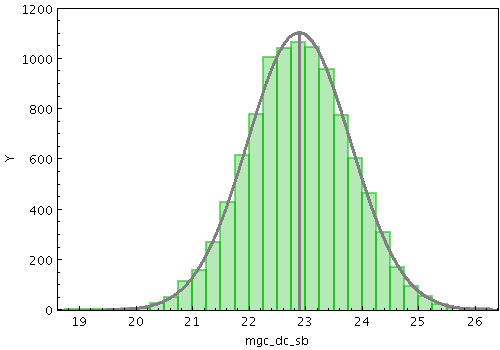
   stilts plot2plane in=mgc_ok.fits x=mgc_dc_sb
                     layer1=histogram color1=green
                     layer2=gaussian color2=grey thick2=3
                     ymax=1200 shadow=false
antialiasN = true|false (Boolean)
[Default: false]
binsizeN = +<width>|-<count> (BinSizer)
When setting this value graphically, you can use either the slider to adjust the bin count or the numeric entry field to fix the bin width.
[Default: -30]
colorN = <rrggbb>|red|blue|... (Color)
The standard plotting colour names are
red, blue, green, grey, magenta, cyan, orange, pink, yellow, black, light_grey, white.
However, many other common colour names (too many to list here)
are also understood.
The list currently contains those colour names understood
by most web browsers,
from AliceBlue to YellowGreen,
listed e.g. in the
Extended color keywords section of
the CSS3 standard.
Alternatively, a six-digit hexadecimal number RRGGBB
may be supplied,
optionally prefixed by "#" or "0x",
giving red, green and blue intensities,
e.g. "ff00ff", "#ff00ff"
or "0xff00ff" for magenta.
[Default: red]
dashN = dot|dash|...|<a,b,...> (float[])
Possible values for dashed lines are
dot, dash, longdash, dotdash.
You can alternatively supply a comma-separated list
of on/off length values such as
"4,2,8,2".
icmdN = <cmds> (ProcessingStep[])
inN.
The value of this parameter is one or more of the filter
commands described in Section 6.1.
If more than one is given, they must be separated by
semicolon characters (";").
This parameter can be repeated multiple times on the same
command line to build up a list of processing steps.
The sequence of commands given in this way
defines the processing pipeline which is performed on the table.
Commands may alternatively be supplied in an external file,
by using the indirection character '@'.
Thus a value of "@filename"
causes the file filename to be read for a list
of filter commands to execute. The commands in the file
may be separated by newline characters and/or semicolons,
and lines which are blank or which start with a
'#' character are ignored.
A backslash character '\' at the end of a line
joins it with the following line.
ifmtN = <in-format> (String)
inN.
The known formats are listed in Section 5.1.1.
This flag can be used if you know what format your
table is in.
If it has the special value
(auto) (the default),
then an attempt will be
made to detect the format of the table automatically.
This cannot always be done correctly however, in which case
the program will exit with an error explaining which
formats were attempted.
This parameter is ignored for scheme-specified tables.
[Default: (auto)]
inN = <table> (StarTable)
-",
meaning standard input.
In this case the input format must be given explicitly
using the ifmtN
parameter.
Note that not all formats can be streamed in this way.:<scheme-name>:<scheme-args>.<" character at the start,
or a "|" character at the end
("<syscmd" or
"syscmd|").
This executes the given pipeline and reads from its
standard output.
This will probably only work on unix-like systems.istreamN = true|false (Boolean)
inN parameter
will be read as a stream.
It is necessary to give the
ifmtN parameter
in this case.
Depending on the required operations and processing mode,
this may cause the read to fail (sometimes it is necessary
to read the table more than once).
It is not normally necessary to set this flag;
in most cases the data will be streamed automatically
if that is the best thing to do.
However it can sometimes result in less resource usage when
processing large files in certain formats (such as VOTable).
This parameter is ignored for scheme-specified tables.
[Default: false]
normaliseN = none|area|unit|maximum|height (Normalisation)
Note that some of the normalisation options may not make much sense with some other parameter values, for instance averaging aggregation modes.
The available options are:
none: No normalisation is performed.area: The total area of histogram bars is normalised to unity. For cumulative plots, this behaves like height.unit: Histogram bars are scaled by the inverse of the bin width in data units. For cumulative plots, this behaves like none.maximum: The height of the tallest histogram bar is normalised to unity. For cumulative plots, this behaves like height.height: The total height of histogram bars is normalised to unity.[Default: none]
showmeanN = true|false (Boolean)
[Default: true]
sidewaysN = true|false (Boolean)
false,
the quantity being accumulated is on the the horizontal axis
and the frequency is represented vertically as usual.
If set true the quantity accumulated
is on the vertical axis,
and the frequency is represented horizontally,
so that the chart is displayed reflected in the X=Y line.
[Default: false]
thickN = <pixels> (Integer)
[Default: 1]
weightN = <num-expr> (String)
The value is a numeric algebraic expression based on column names as described in Section 10.
xN = <num-expr> (String)
The value is a numeric algebraic expression based on column names as described in Section 10.
function
Plots an analytic function. This layer is currently only available for the Plane plots (including histogram).
Usage Overview:
   layerN=function axisN=Horizontal|Vertical xnameN=<name> fexprN=<expr>
                   colorN=<rrggbb>|red|blue|... thickN=<pixels>
                   dashN=dot|dash|...|<a,b,...> antialiasN=true|false
All the parameters listed here
affect only the relevant layer,
identified by the suffix
N.
Example:
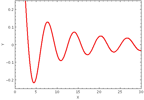
   stilts plot2plane layer1=function fexpr1=sin(x)/x thick1=3
                     xmin=0 xmax=30 ymin=-0.25 ymax=0.25
antialiasN = true|false (Boolean)
[Default: false]
axisN = Horizontal|Vertical (FuncAxis)
Horizontal and
Vertical.
[Default: Horizontal]
colorN = <rrggbb>|red|blue|... (Color)
The standard plotting colour names are
red, blue, green, grey, magenta, cyan, orange, pink, yellow, black, light_grey, white.
However, many other common colour names (too many to list here)
are also understood.
The list currently contains those colour names understood
by most web browsers,
from AliceBlue to YellowGreen,
listed e.g. in the
Extended color keywords section of
the CSS3 standard.
Alternatively, a six-digit hexadecimal number RRGGBB
may be supplied,
optionally prefixed by "#" or "0x",
giving red, green and blue intensities,
e.g. "ff00ff", "#ff00ff"
or "0xff00ff" for magenta.
[Default: red]
dashN = dot|dash|...|<a,b,...> (float[])
Possible values for dashed lines are
dot, dash, longdash, dotdash.
You can alternatively supply a comma-separated list
of on/off length values such as
"4,2,8,2".
fexprN = <expr> (String)
thickN = <pixels> (Integer)
[Default: 1]
xnameN = <name> (String)
x for a horizontal independent variable and
y for a vertical independent variable,
but any string that is a legal expression language identifier
(starts with a letter, continues with letters, numbers,
underscores) can be used.
[Default: x]
skyvector
Plots directed lines from the data position given delta values for the coordinates The plotted markers are typically little arrows, but there are other options.
The dimensions of the plotted vectors
are given by the
dlon and dlat
coordinates.
The units of these values are specified using the
unit option.
If only the relative rather than the absolute sizes
are required on the plot,
or if the units are not known,
the special value
unit=scaled
may be used;
this applies a non-physical scaling factor
to make the vectors appear at some reasonable size
in the plot.
When unit=scaled
vectors will keep approximately the same screen size
during zoom operations;
when one of the angular units is chosen, they will keep
the same size in data coordinates.
Additionally, the
scale option
may be used to scale all the plotted vectors
by a given factor to make them all larger or smaller.
Usage Overview:
   layerN=skyvector arrowN=small_arrow|medium_arrow|... thickN=<int-value>
                    scaleN=<number>
                    unitN=scaled|radian|degree|minute|arcsec|mas|uas
                    shadingN=auto|flat|translucent|transparent|density|aux|weighted|paux|pweighted <shade-paramsN>
                    lonN=<deg-expr> latN=<deg-expr> dlonN=<num-expr>
                    dlatN=<num-expr> inN=<table> ifmtN=<in-format>
                    istreamN=true|false icmdN=<cmds>
All the parameters listed here
affect only the relevant layer,
identified by the suffix
N.
Example:
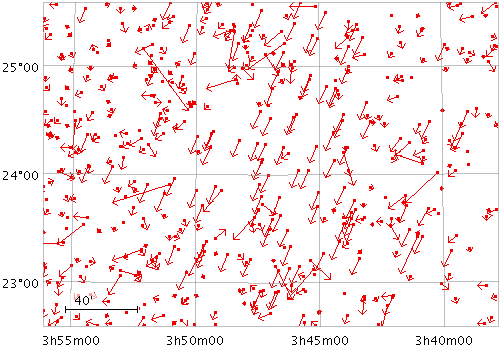
   stilts plot2sky in=tgas_source.fits lon=ra lat=dec
                   layer1=mark
                   layer2=skyvector
                   dlon2=pmra dlat2=pmdec unit2=scaled scale2=6 arrow2=medium_arrow
                   clon=56.75 clat=24.10 radius=1.5
arrowN = small_arrow|medium_arrow|... (MultiPointShape)
The available options are:
small_arrow
medium_arrow
large_arrow
small_open_dart
medium_open_dart
large_open_dart
small_filled_dart
medium_filled_dart
large_filled_dart
lines
capped_lines
[Default: small_arrow]
dlatN = <num-expr> (String)
unit option.
The value is a numeric algebraic expression based on column names as described in Section 10.
dlonN = <num-expr> (String)
unit option.
The value is a numeric algebraic expression based on column names as described in Section 10.
icmdN = <cmds> (ProcessingStep[])
inN.
The value of this parameter is one or more of the filter
commands described in Section 6.1.
If more than one is given, they must be separated by
semicolon characters (";").
This parameter can be repeated multiple times on the same
command line to build up a list of processing steps.
The sequence of commands given in this way
defines the processing pipeline which is performed on the table.
Commands may alternatively be supplied in an external file,
by using the indirection character '@'.
Thus a value of "@filename"
causes the file filename to be read for a list
of filter commands to execute. The commands in the file
may be separated by newline characters and/or semicolons,
and lines which are blank or which start with a
'#' character are ignored.
A backslash character '\' at the end of a line
joins it with the following line.
ifmtN = <in-format> (String)
inN.
The known formats are listed in Section 5.1.1.
This flag can be used if you know what format your
table is in.
If it has the special value
(auto) (the default),
then an attempt will be
made to detect the format of the table automatically.
This cannot always be done correctly however, in which case
the program will exit with an error explaining which
formats were attempted.
This parameter is ignored for scheme-specified tables.
[Default: (auto)]
inN = <table> (StarTable)
-",
meaning standard input.
In this case the input format must be given explicitly
using the ifmtN
parameter.
Note that not all formats can be streamed in this way.:<scheme-name>:<scheme-args>.<" character at the start,
or a "|" character at the end
("<syscmd" or
"syscmd|").
This executes the given pipeline and reads from its
standard output.
This will probably only work on unix-like systems.istreamN = true|false (Boolean)
inN parameter
will be read as a stream.
It is necessary to give the
ifmtN parameter
in this case.
Depending on the required operations and processing mode,
this may cause the read to fail (sometimes it is necessary
to read the table more than once).
It is not normally necessary to set this flag;
in most cases the data will be streamed automatically
if that is the best thing to do.
However it can sometimes result in less resource usage when
processing large files in certain formats (such as VOTable).
This parameter is ignored for scheme-specified tables.
[Default: false]
latN = <deg-expr> (String)
The value is a numeric algebraic expression based on column names as described in Section 10.
lonN = <deg-expr> (String)
The value is a numeric algebraic expression based on column names as described in Section 10.
scaleN = <number> (Double)
The main purpose of this option is to tweak
the visible sizes of the plotted markers for better visibility.
The unit option
should be used to account for the units in which the
angular extent coordinates are supplied.
If the markers are supposed to be plotted with their
absolute angular extents visible, this option should be set
to its default value of 1.
[Default: 1]
shadingN = auto|flat|translucent|transparent|density|aux|weighted|paux|pweighted <shade-paramsN> (ShapeMode)
[Default: auto]
thickN = <int-value> (Integer)
[Default: 0]
unitN = scaled|radian|degree|minute|arcsec|mas|uas (AngleUnit)
scaled is given
then a non-physical scaling is applied to the
input values to make the the largest markers
appear at a reasonable size (a few tens of pixels)
in the plot.
Note that the actual plotted size of the markers
can also be scaled using the
scale option;
these two work together to determine the actual plotted sizes.
The available options are:
scaled: a non-physical scaling is applied
based on the size of values present
radian: radiansdegree: degreesminute: arcminutesarcsec: arcsecondsmas: milli-arcsecondsuas: micro-arcseconds[Default: degree]
skyellipse
Plots an ellipse (or rectangle, triangle, or other similar figure) defined by two principal radii and an optional angle of rotation, the so-called position angle. This angle, if specified, is in degrees and gives the angle from the North pole towards the direction of increasing longitude on the longitude axis.
The dimensions of the plotted ellipses
are given by the
ra and rb
coordinates.
The units of these values are specified using the
unit option.
If only the relative rather than the absolute sizes
are required on the plot,
or if the units are not known,
the special value
unit=scaled
may be used;
this applies a non-physical scaling factor
to make the ellipses appear at some reasonable size
in the plot.
When unit=scaled
ellipses will keep approximately the same screen size
during zoom operations;
when one of the angular units is chosen, they will keep
the same size in data coordinates.
Additionally, the
scale option
may be used to scale all the plotted ellipses
by a given factor to make them all larger or smaller.
Usage Overview:
   layerN=skyellipse ellipseN=ellipse|crosshair_ellipse|... thickN=<int-value>
                     scaleN=<number>
                     unitN=scaled|radian|degree|minute|arcsec|mas|uas
                     shadingN=auto|flat|translucent|transparent|density|aux|weighted|paux|pweighted <shade-paramsN>
                     lonN=<deg-expr> latN=<deg-expr> raN=<num-expr>
                     rbN=<num-expr> posangN=<deg-expr> inN=<table>
                     ifmtN=<in-format> istreamN=true|false icmdN=<cmds>
All the parameters listed here
affect only the relevant layer,
identified by the suffix
N.
Example:
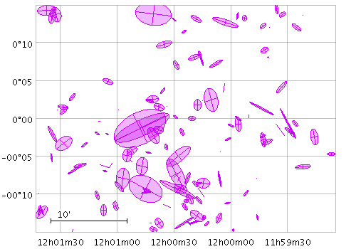
   stilts plot2sky in=mgc_ok.fits
                   lon=mgc_alpha_j2000 lat=mgc_delta_j2000
                   ra=bulge_re rb=bulge_re*bulge_e unit=arcsec posang=bulge_pa
                   scale=10 color=#cc00ff
                   layer1=skyellipse ellipse1=filled_ellipse shading1=transparent opaque1=4
                   layer2=skyellipse ellipse2=crosshair_ellipse
                   clon=180.1 clat=0 radius=0.25
ellipseN = ellipse|crosshair_ellipse|... (MultiPointShape)
The available options are:
ellipse
crosshair_ellipse
filled_ellipse
rectangle
crosshair_rectangle
filled_rectangle
open_triangle
filled_triangle
lines
capped_lines
arrows
[Default: ellipse]
icmdN = <cmds> (ProcessingStep[])
inN.
The value of this parameter is one or more of the filter
commands described in Section 6.1.
If more than one is given, they must be separated by
semicolon characters (";").
This parameter can be repeated multiple times on the same
command line to build up a list of processing steps.
The sequence of commands given in this way
defines the processing pipeline which is performed on the table.
Commands may alternatively be supplied in an external file,
by using the indirection character '@'.
Thus a value of "@filename"
causes the file filename to be read for a list
of filter commands to execute. The commands in the file
may be separated by newline characters and/or semicolons,
and lines which are blank or which start with a
'#' character are ignored.
A backslash character '\' at the end of a line
joins it with the following line.
ifmtN = <in-format> (String)
inN.
The known formats are listed in Section 5.1.1.
This flag can be used if you know what format your
table is in.
If it has the special value
(auto) (the default),
then an attempt will be
made to detect the format of the table automatically.
This cannot always be done correctly however, in which case
the program will exit with an error explaining which
formats were attempted.
This parameter is ignored for scheme-specified tables.
[Default: (auto)]
inN = <table> (StarTable)
-",
meaning standard input.
In this case the input format must be given explicitly
using the ifmtN
parameter.
Note that not all formats can be streamed in this way.:<scheme-name>:<scheme-args>.<" character at the start,
or a "|" character at the end
("<syscmd" or
"syscmd|").
This executes the given pipeline and reads from its
standard output.
This will probably only work on unix-like systems.istreamN = true|false (Boolean)
inN parameter
will be read as a stream.
It is necessary to give the
ifmtN parameter
in this case.
Depending on the required operations and processing mode,
this may cause the read to fail (sometimes it is necessary
to read the table more than once).
It is not normally necessary to set this flag;
in most cases the data will be streamed automatically
if that is the best thing to do.
However it can sometimes result in less resource usage when
processing large files in certain formats (such as VOTable).
This parameter is ignored for scheme-specified tables.
[Default: false]
latN = <deg-expr> (String)
The value is a numeric algebraic expression based on column names as described in Section 10.
lonN = <deg-expr> (String)
The value is a numeric algebraic expression based on column names as described in Section 10.
posangN = <deg-expr> (String)
The value is a numeric algebraic expression based on column names as described in Section 10.
raN = <num-expr> (String)
unit option.
The value is a numeric algebraic expression based on column names as described in Section 10.
rbN = <num-expr> (String)
unit option.
If this value is blank, the two radii will be assumed equal,
i.e. the ellipses will be circles.
The value is a numeric algebraic expression based on column names as described in Section 10.
scaleN = <number> (Double)
The main purpose of this option is to tweak
the visible sizes of the plotted markers for better visibility.
The unit option
should be used to account for the units in which the
angular extent coordinates are supplied.
If the markers are supposed to be plotted with their
absolute angular extents visible, this option should be set
to its default value of 1.
[Default: 1]
shadingN = auto|flat|translucent|transparent|density|aux|weighted|paux|pweighted <shade-paramsN> (ShapeMode)
[Default: auto]
thickN = <int-value> (Integer)
[Default: 0]
unitN = scaled|radian|degree|minute|arcsec|mas|uas (AngleUnit)
scaled is given
then a non-physical scaling is applied to the
input values to make the the largest markers
appear at a reasonable size (a few tens of pixels)
in the plot.
Note that the actual plotted size of the markers
can also be scaled using the
scale option;
these two work together to determine the actual plotted sizes.
The available options are:
scaled: a non-physical scaling is applied
based on the size of values present
radian: radiansdegree: degreesminute: arcminutesarcsec: arcsecondsmas: milli-arcsecondsuas: micro-arcseconds[Default: degree]
skycorr
Plots an error ellipse (or rectangle or other similar figure) on the sky defined by errors in the longitude and latitude directions, and a correlation between the two errors.
The error in longitude is considered to be premultiplied by the cosine of the latitude, i.e. both errors correspond to angular distances along a great circle.
The supplied correlation is a dimensionless value in the range -1..+1 and is equal to the covariance divided by the product of the lon and lat errors. The covariance matrix is thus:
    [  lonerr*lonerr       lonerr*laterr*corr  ]
    [  lonerr*laterr*corr  laterr*laterr       ]
The dimensions of the plotted ellipses
are given by the
lonerr and laterr
coordinates.
The units of these values are specified using the
unit option.
If only the relative rather than the absolute sizes
are required on the plot,
or if the units are not known,
the special value
unit=scaled
may be used;
this applies a non-physical scaling factor
to make the ellipses appear at some reasonable size
in the plot.
When unit=scaled
ellipses will keep approximately the same screen size
during zoom operations;
when one of the angular units is chosen, they will keep
the same size in data coordinates.
Additionally, the
scale option
may be used to scale all the plotted ellipses
by a given factor to make them all larger or smaller.
This plot type is suitable for use with the
ra_error, dec_error and
ra_dec_corr columns
in the Gaia source catalogue.
Note that Gaia positional errors are generally quoted
in milli-arcseconds, so you should set
unit=mas.
Note also that in most plots Gaia positional errors
are much too small to see!
Usage Overview:
   layerN=skycorr ellipseN=ellipse|crosshair_ellipse|... thickN=<int-value>
                  scaleN=<number>
                  unitN=scaled|radian|degree|minute|arcsec|mas|uas
                  shadingN=auto|flat|translucent|transparent|density|aux|weighted|paux|pweighted <shade-paramsN>
                  lonN=<deg-expr> latN=<deg-expr> lonerrN=<num-expr>
                  laterrN=<num-expr> corrN=<num-expr> inN=<table>
                  ifmtN=<in-format> istreamN=true|false icmdN=<cmds>
All the parameters listed here
affect only the relevant layer,
identified by the suffix
N.
Example:
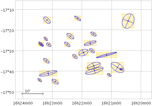
   stilts plot2sky in=tgas_source.fits
                   lon=ra lat=dec
                   icmd='select ra>245.1&&ra<245.9&&dec>-17.8&&dec<-17.2'
                   color=blue
                   layer1=mark
                   unit=mas scale=2e5
                   ra2=ra_error rb2=dec_error posang2=90
                   color2=orange shading2=transparent
                   layer2a=skyellipse ellipse2a=filled_rectangle opaque2a=6
                   layer2b=skyellipse ellipse2b=crosshair_rectangle opaque2b=2
                   layer3=skycorr
                   lonerr3=ra_error laterr3=dec_error corr3=ra_dec_corr
                   ellipse3=crosshair_ellipse
corrN = <num-expr> (String)
ra_dec_corr value
supplied in the Gaia source catalogue.
The value is a numeric algebraic expression based on column names as described in Section 10.
ellipseN = ellipse|crosshair_ellipse|... (MultiPointShape)
The available options are:
ellipse
crosshair_ellipse
filled_ellipse
rectangle
crosshair_rectangle
filled_rectangle
open_triangle
filled_triangle
lines
capped_lines
arrows
[Default: ellipse]
icmdN = <cmds> (ProcessingStep[])
inN.
The value of this parameter is one or more of the filter
commands described in Section 6.1.
If more than one is given, they must be separated by
semicolon characters (";").
This parameter can be repeated multiple times on the same
command line to build up a list of processing steps.
The sequence of commands given in this way
defines the processing pipeline which is performed on the table.
Commands may alternatively be supplied in an external file,
by using the indirection character '@'.
Thus a value of "@filename"
causes the file filename to be read for a list
of filter commands to execute. The commands in the file
may be separated by newline characters and/or semicolons,
and lines which are blank or which start with a
'#' character are ignored.
A backslash character '\' at the end of a line
joins it with the following line.
ifmtN = <in-format> (String)
inN.
The known formats are listed in Section 5.1.1.
This flag can be used if you know what format your
table is in.
If it has the special value
(auto) (the default),
then an attempt will be
made to detect the format of the table automatically.
This cannot always be done correctly however, in which case
the program will exit with an error explaining which
formats were attempted.
This parameter is ignored for scheme-specified tables.
[Default: (auto)]
inN = <table> (StarTable)
-",
meaning standard input.
In this case the input format must be given explicitly
using the ifmtN
parameter.
Note that not all formats can be streamed in this way.:<scheme-name>:<scheme-args>.<" character at the start,
or a "|" character at the end
("<syscmd" or
"syscmd|").
This executes the given pipeline and reads from its
standard output.
This will probably only work on unix-like systems.istreamN = true|false (Boolean)
inN parameter
will be read as a stream.
It is necessary to give the
ifmtN parameter
in this case.
Depending on the required operations and processing mode,
this may cause the read to fail (sometimes it is necessary
to read the table more than once).
It is not normally necessary to set this flag;
in most cases the data will be streamed automatically
if that is the best thing to do.
However it can sometimes result in less resource usage when
processing large files in certain formats (such as VOTable).
This parameter is ignored for scheme-specified tables.
[Default: false]
latN = <deg-expr> (String)
The value is a numeric algebraic expression based on column names as described in Section 10.
laterrN = <num-expr> (String)
unit option.
The value is a numeric algebraic expression based on column names as described in Section 10.
lonN = <deg-expr> (String)
The value is a numeric algebraic expression based on column names as described in Section 10.
lonerrN = <num-expr> (String)
unit option.
The value is a numeric algebraic expression based on column names as described in Section 10.
scaleN = <number> (Double)
The main purpose of this option is to tweak
the visible sizes of the plotted markers for better visibility.
The unit option
should be used to account for the units in which the
angular extent coordinates are supplied.
If the markers are supposed to be plotted with their
absolute angular extents visible, this option should be set
to its default value of 1.
[Default: 1]
shadingN = auto|flat|translucent|transparent|density|aux|weighted|paux|pweighted <shade-paramsN> (ShapeMode)
[Default: auto]
thickN = <int-value> (Integer)
[Default: 0]
unitN = scaled|radian|degree|minute|arcsec|mas|uas (AngleUnit)
scaled is given
then a non-physical scaling is applied to the
input values to make the the largest markers
appear at a reasonable size (a few tens of pixels)
in the plot.
Note that the actual plotted size of the markers
can also be scaled using the
scale option;
these two work together to determine the actual plotted sizes.
The available options are:
scaled: a non-physical scaling is applied
based on the size of values present
radian: radiansdegree: degreesminute: arcminutesarcsec: arcsecondsmas: milli-arcsecondsuas: micro-arcseconds[Default: degree]
skydensity
Plots a density map on the sky. The grid on which the values are drawn uses the HEALPix tesselation, with a configurable resolution. You can optionally use a weighting for the points, and you can configure how the points are combined to produce the output pixel values.
The way that data values are mapped to colours is usually controlled by options at the level of the plot itself, rather than by per-layer configuration.
Usage Overview:
   layerN=skydensity levelN=<-rel-level|+abs-level>
                     combineN=sum|sum-per-unit|count|...
                     perunitN=steradian|degree2|arcmin2|arcsec2|mas2|uas2
                     transparencyN=0..1 lonN=<deg-expr> latN=<deg-expr>
                     weightN=<num-expr> inN=<table> ifmtN=<in-format>
                     istreamN=true|false icmdN=<cmds>
All the parameters listed here
affect only the relevant layer,
identified by the suffix
N.
Example:
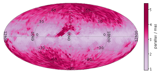
   stilts plot2sky in=tgas_source.fits lon=l lat=b
                   layer1=skydensity weight1=parallax combine1=mean level1=4
                   projection=aitoff auxmap=PuRd auxfunc=histogram
                   xpix=540 ypix=250
combineN = sum|sum-per-unit|count|... (Combiner)
weight
is left blank, a weighting of unity is assumed.
For density-like values
(count-per-unit,
sum-per-unit)
the scaling is additionally influenced by the
perunit parameter.
The available options are:
sum: the sum of all the combined values per binsum-per-unit: the sum of all the combined values per unit of bin sizecount: the number of non-blank values per bin (weight is ignored)count-per-unit: the number of non-blank values per unit of bin size (weight is ignored)mean: the mean of the combined valuesmedian: the medianq1: first quartileq3: third quartilemin: the minimum of all the combined valuesmax: the maximum of all the combined valuesstdev: the sample standard deviation of the combined valuesstdev_pop: the population standard deviation of the combined valueshit: 1 if any values present, NaN otherwise (weight is ignored)[Default: sum-per-unit]
icmdN = <cmds> (ProcessingStep[])
inN.
The value of this parameter is one or more of the filter
commands described in Section 6.1.
If more than one is given, they must be separated by
semicolon characters (";").
This parameter can be repeated multiple times on the same
command line to build up a list of processing steps.
The sequence of commands given in this way
defines the processing pipeline which is performed on the table.
Commands may alternatively be supplied in an external file,
by using the indirection character '@'.
Thus a value of "@filename"
causes the file filename to be read for a list
of filter commands to execute. The commands in the file
may be separated by newline characters and/or semicolons,
and lines which are blank or which start with a
'#' character are ignored.
A backslash character '\' at the end of a line
joins it with the following line.
ifmtN = <in-format> (String)
inN.
The known formats are listed in Section 5.1.1.
This flag can be used if you know what format your
table is in.
If it has the special value
(auto) (the default),
then an attempt will be
made to detect the format of the table automatically.
This cannot always be done correctly however, in which case
the program will exit with an error explaining which
formats were attempted.
This parameter is ignored for scheme-specified tables.
[Default: (auto)]
inN = <table> (StarTable)
-",
meaning standard input.
In this case the input format must be given explicitly
using the ifmtN
parameter.
Note that not all formats can be streamed in this way.:<scheme-name>:<scheme-args>.<" character at the start,
or a "|" character at the end
("<syscmd" or
"syscmd|").
This executes the given pipeline and reads from its
standard output.
This will probably only work on unix-like systems.istreamN = true|false (Boolean)
inN parameter
will be read as a stream.
It is necessary to give the
ifmtN parameter
in this case.
Depending on the required operations and processing mode,
this may cause the read to fail (sometimes it is necessary
to read the table more than once).
It is not normally necessary to set this flag;
in most cases the data will be streamed automatically
if that is the best thing to do.
However it can sometimes result in less resource usage when
processing large files in certain formats (such as VOTable).
This parameter is ignored for scheme-specified tables.
[Default: false]
latN = <deg-expr> (String)
The value is a numeric algebraic expression based on column names as described in Section 10.
levelN = <-rel-level|+abs-level> (Integer)
If the supplied value is a non-negative integer, it gives the absolute level to use; at level 0 there are 12 pixels on the sky, and the count multiplies by 4 for each increment.
If the value is negative, it represents a relative level; it is approximately the (negative) number of screen pixels along one side of a HEALPix sky pixel. In this case the actual HEALPix level will depend on the current zoom.
[Default: -3]
lonN = <deg-expr> (String)
The value is a numeric algebraic expression based on column names as described in Section 10.
perunitN = steradian|degree2|arcmin2|arcsec2|mas2|uas2 (SolidAngleUnit)
combine=count-per-unit or
sum-per-unit).
If the Combination mode is calculating values per unit area,
this configures the area scale in question.
For non-density-like combination modes
(e.g. combine=sum or
mean)
it has no effect.
The available options are:
steradian: (180/Pi)^2 deg^2degree2: square degreesarcmin2: square arcminute, (1/60)^2 deg^2arcsec2: square arcsecond, (1/3600)^2 deg^2mas2: square milliarcsecond, (.001/3600)^2 deg^2uas2: square microarcsecond, (1e-6/3600)^2 deg^2[Default: degree2]
transparencyN = 0..1 (Double)
[Default: 0]
weightN = <num-expr> (String)
The value is a numeric algebraic expression based on column names as described in Section 10.
skyvecfield
Plots a field of arrows on a HEALPix grid corresponding to the aggregated (typically averaged) value of a 2-d vector quantity such as proper motion for the points in each cell.
Currently, the visible length of the vectors is dependent
on the size of the grid; they are sized to appear with a
length comparable to the size of the HEALPix cells.
Units of the values specified are therefore not relevant.
This length can be adjusted by use of the
scale option.
By default, the absolute values of the vectors are plotted.
However, if the
relative option
is set, the mean vector value averaged over the visible plot area
will be calculated and subtracted from all the plotted vectors.
The effect of this is to show local variations rather than
absolute values of the vectors over the visible area.
Usage Overview:
   layerN=skyvecfield colorN=<rrggbb>|red|blue|...
                      arrowN=small_arrow|medium_arrow|... thickN=<int-value>
                      scaleN=<number> levelN=<-rel-level|+abs-level>
                      combineN=mean|sum relativeN=true|false lonN=<deg-expr>
                      latN=<deg-expr> vlonN=<num-expr> vlatN=<num-expr>
                      weightN=<num-expr> inN=<table> ifmtN=<in-format>
                      istreamN=true|false icmdN=<cmds>
All the parameters listed here
affect only the relevant layer,
identified by the suffix
N.
Example:
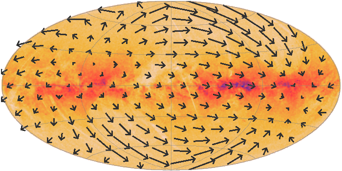
   stilts plot2sky xpix=700 ypix=350 projection=aitoff datasys=equatorial viewsys=galactic labelpos=none
                   in=tgas_source.fits lon=ra lat=dec
                   layer_1=mark shading_1=density densemap_1=sunset densefunc_1=sqrt
                   layer_2=skyvecfield vlon_2=pmra vlat_2=pmdec color_2=#303030 arrow_2=large_arrow thick_2=1
arrowN = small_arrow|medium_arrow|... (MultiPointShape)
The available options are:
small_arrow
medium_arrow
large_arrow
small_open_dart
medium_open_dart
large_open_dart
small_filled_dart
medium_filled_dart
large_filled_dart
lines
capped_lines
[Default: small_arrow]
colorN = <rrggbb>|red|blue|... (Color)
The standard plotting colour names are
red, blue, green, grey, magenta, cyan, orange, pink, yellow, black, light_grey, white.
However, many other common colour names (too many to list here)
are also understood.
The list currently contains those colour names understood
by most web browsers,
from AliceBlue to YellowGreen,
listed e.g. in the
Extended color keywords section of
the CSS3 standard.
Alternatively, a six-digit hexadecimal number RRGGBB
may be supplied,
optionally prefixed by "#" or "0x",
giving red, green and blue intensities,
e.g. "ff00ff", "#ff00ff"
or "0xff00ff" for magenta.
[Default: red]
combineN = mean|sum (Combiner)
The available options are:
mean: the mean of the combined valuessum: the sum of all the combined values per bin[Default: mean]
icmdN = <cmds> (ProcessingStep[])
inN.
The value of this parameter is one or more of the filter
commands described in Section 6.1.
If more than one is given, they must be separated by
semicolon characters (";").
This parameter can be repeated multiple times on the same
command line to build up a list of processing steps.
The sequence of commands given in this way
defines the processing pipeline which is performed on the table.
Commands may alternatively be supplied in an external file,
by using the indirection character '@'.
Thus a value of "@filename"
causes the file filename to be read for a list
of filter commands to execute. The commands in the file
may be separated by newline characters and/or semicolons,
and lines which are blank or which start with a
'#' character are ignored.
A backslash character '\' at the end of a line
joins it with the following line.
ifmtN = <in-format> (String)
inN.
The known formats are listed in Section 5.1.1.
This flag can be used if you know what format your
table is in.
If it has the special value
(auto) (the default),
then an attempt will be
made to detect the format of the table automatically.
This cannot always be done correctly however, in which case
the program will exit with an error explaining which
formats were attempted.
This parameter is ignored for scheme-specified tables.
[Default: (auto)]
inN = <table> (StarTable)
-",
meaning standard input.
In this case the input format must be given explicitly
using the ifmtN
parameter.
Note that not all formats can be streamed in this way.:<scheme-name>:<scheme-args>.<" character at the start,
or a "|" character at the end
("<syscmd" or
"syscmd|").
This executes the given pipeline and reads from its
standard output.
This will probably only work on unix-like systems.istreamN = true|false (Boolean)
inN parameter
will be read as a stream.
It is necessary to give the
ifmtN parameter
in this case.
Depending on the required operations and processing mode,
this may cause the read to fail (sometimes it is necessary
to read the table more than once).
It is not normally necessary to set this flag;
in most cases the data will be streamed automatically
if that is the best thing to do.
However it can sometimes result in less resource usage when
processing large files in certain formats (such as VOTable).
This parameter is ignored for scheme-specified tables.
[Default: false]
latN = <deg-expr> (String)
The value is a numeric algebraic expression based on column names as described in Section 10.
levelN = <-rel-level|+abs-level> (Integer)
If the supplied value is a non-negative integer, it gives the absolute level to use; at level 0 there are 12 pixels on the sky, and the count multiplies by 4 for each increment.
If the value is negative, it represents a relative level; it is approximately the (negative) number of screen pixels along one side of a HEALPix sky pixel. In this case the actual HEALPix level will depend on the current zoom.
[Default: -4]
lonN = <deg-expr> (String)
The value is a numeric algebraic expression based on column names as described in Section 10.
relativeN = true|false (Boolean)
[Default: false]
scaleN = <number> (Double)
[Default: 1]
thickN = <int-value> (Integer)
[Default: 0]
vlatN = <num-expr> (String)
The value is a numeric algebraic expression based on column names as described in Section 10.
vlonN = <num-expr> (String)
The value is a numeric algebraic expression based on column names as described in Section 10.
weightN = <num-expr> (String)
The value is a numeric algebraic expression based on column names as described in Section 10.
healpix
Plots a table representing HEALPix pixels on the sky. Each row represents a single HEALPix tile, and a value from that row is used to colour the corresponding region of the sky plot.
The way that data values are mapped to colours is usually controlled by options at the level of the plot itself, rather than by per-layer configuration.
Usage Overview:
   layerN=healpix datalevelN=<int-value> datasysN=<value> degradeN=<int-value>
                  combineN=sum|sum-per-unit|count|...
                  perunitN=steradian|degree2|arcmin2|arcsec2|mas2|uas2
                  transparencyN=0..1 healpixN=<num-expr> valueN=<num-expr>
                  inN=<table> ifmtN=<in-format> istreamN=true|false
                  icmdN=<cmds>
All the parameters listed here
affect only the relevant layer,
identified by the suffix
N.
Example:
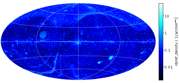
   stilts plot2sky layer1=healpix in1=simbad-hpx8.fits healpix1=HPX8 value1=NBREF
                   datalevel1=8 degrade1=2 combine=sum-per-unit perunit=arcmin2
                   projection=aitoff datasys1=equatorial viewsys=galactic labelpos=none gridcolor=beige
                   auxfunc=log auxmap=cold auxflip=true auxclip=0,1
                   xpix=600 ypix=280
combineN = sum|sum-per-unit|count|... (Combiner)
degrade>0.
For density-like values
(count-per-unit,
sum-per-unit)
the scaling is additionally influenced by the
perunit
parameter.
The available options are:
sum: the sum of all the combined values per binsum-per-unit: the sum of all the combined values per unit of bin sizecount: the number of non-blank values per bin (weight is ignored)count-per-unit: the number of non-blank values per unit of bin size (weight is ignored)mean: the mean of the combined valuesmedian: the medianq1: first quartileq3: third quartilemin: the minimum of all the combined valuesmax: the maximum of all the combined valuesstdev: the sample standard deviation of the combined valuesstdev_pop: the population standard deviation of the combined valueshit: 1 if any values present, NaN otherwise (weight is ignored)[Default: mean]
datalevelN = <int-value> (Integer)
[Default: -1]
datasysN = <value> (SkySys)
[Default: equatorial]
degradeN = <int-value> (Integer)
degrade input tiles.
The way that values are combined within each painted tile
is controlled by the
combine value.
[Default: 0]
healpixN = <num-expr> (String)
The value is a numeric algebraic expression based on column names as described in Section 10.
icmdN = <cmds> (ProcessingStep[])
inN.
The value of this parameter is one or more of the filter
commands described in Section 6.1.
If more than one is given, they must be separated by
semicolon characters (";").
This parameter can be repeated multiple times on the same
command line to build up a list of processing steps.
The sequence of commands given in this way
defines the processing pipeline which is performed on the table.
Commands may alternatively be supplied in an external file,
by using the indirection character '@'.
Thus a value of "@filename"
causes the file filename to be read for a list
of filter commands to execute. The commands in the file
may be separated by newline characters and/or semicolons,
and lines which are blank or which start with a
'#' character are ignored.
A backslash character '\' at the end of a line
joins it with the following line.
ifmtN = <in-format> (String)
inN.
The known formats are listed in Section 5.1.1.
This flag can be used if you know what format your
table is in.
If it has the special value
(auto) (the default),
then an attempt will be
made to detect the format of the table automatically.
This cannot always be done correctly however, in which case
the program will exit with an error explaining which
formats were attempted.
This parameter is ignored for scheme-specified tables.
[Default: (auto)]
inN = <table> (StarTable)
-",
meaning standard input.
In this case the input format must be given explicitly
using the ifmtN
parameter.
Note that not all formats can be streamed in this way.:<scheme-name>:<scheme-args>.<" character at the start,
or a "|" character at the end
("<syscmd" or
"syscmd|").
This executes the given pipeline and reads from its
standard output.
This will probably only work on unix-like systems.istreamN = true|false (Boolean)
inN parameter
will be read as a stream.
It is necessary to give the
ifmtN parameter
in this case.
Depending on the required operations and processing mode,
this may cause the read to fail (sometimes it is necessary
to read the table more than once).
It is not normally necessary to set this flag;
in most cases the data will be streamed automatically
if that is the best thing to do.
However it can sometimes result in less resource usage when
processing large files in certain formats (such as VOTable).
This parameter is ignored for scheme-specified tables.
[Default: false]
perunitN = steradian|degree2|arcmin2|arcsec2|mas2|uas2 (SolidAngleUnit)
combine=count-per-unit or
sum-per-unit).
If the Combination mode is calculating values per unit area,
this configures the area scale in question.
For non-density-like combination modes
(e.g. combine=sum or
mean)
it has no effect.
The available options are:
steradian: (180/Pi)^2 deg^2degree2: square degreesarcmin2: square arcminute, (1/60)^2 deg^2arcsec2: square arcsecond, (1/3600)^2 deg^2mas2: square milliarcsecond, (.001/3600)^2 deg^2uas2: square microarcsecond, (1e-6/3600)^2 deg^2[Default: degree2]
transparencyN = 0..1 (Double)
[Default: 0]
valueN = <num-expr> (String)
The value is a numeric algebraic expression based on column names as described in Section 10.
skygrid
Plots an additional axis grid on the celestial sphere.
This can be overlaid on the default sky axis grid
so that axes for multiple sky coordinate systems
are simultaneously visible.
The plots are done relative to the View sky system
(viewsys parameter)
defined for the plot as a whole.
Note that some of the configuration items for this plotter, such as grid line antialiasing and the decimal/sexagesimal flag, are inherited from the values set for the main sky plot grid.
Usage Overview:
   layerN=skygrid gridsysN=equatorial|galactic|supergalactic|ecliptic
                  gridcolorN=<rrggbb>|red|blue|... transparencyN=0..1
                  labelposN=Internal|None loncrowdN=<number> latcrowdN=<number>
All the parameters listed here
affect only the relevant layer,
identified by the suffix
N.
Example:
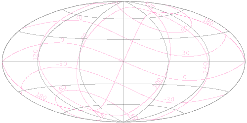
   stilts plot2sky xpix=500 ypix=250 projection=aitoff
                   viewsys=equatorial labelpos=none sex=false
                   layer1=skygrid gridsys1=ecliptic gridcolor1=HotPink transparency1=0.7 labelpos1=internal
gridcolorN = <rrggbb>|red|blue|... (Color)
The standard plotting colour names are
red, blue, green, grey, magenta, cyan, orange, pink, yellow, black, light_grey, white.
However, many other common colour names (too many to list here)
are also understood.
The list currently contains those colour names understood
by most web browsers,
from AliceBlue to YellowGreen,
listed e.g. in the
Extended color keywords section of
the CSS3 standard.
Alternatively, a six-digit hexadecimal number RRGGBB
may be supplied,
optionally prefixed by "#" or "0x",
giving red, green and blue intensities,
e.g. "ff00ff", "#ff00ff"
or "0xff00ff" for magenta.
[Default: grey]
gridsysN = equatorial|galactic|supergalactic|ecliptic (SkySys)
viewsys parameter
defined for the plot as a whole
to determine what grid lines to plot.
The available options are:
equatorial: J2000 equatorial systemgalactic: IAU 1958 galactic systemsupergalactic: De Vaucouleurs supergalactic systemecliptic: ecliptic system based on conversion at 2000.0[Default: equatorial]
labelposN = Internal|None (SkyAxisLabeller)
The available options are:
Internal: Labels are drawn inside the plot boundsNone: Axes are not labelled[Default: Internal]
latcrowdN = <number> (Double)
[Default: 1]
loncrowdN = <number> (Double)
[Default: 1]
transparencyN = 0..1 (Double)
[Default: 0]
xyzvector
Plots directed lines from the data position given delta values for the coordinates. The plotted markers are typically little arrows, but there are other options.
In some cases the supplied data values
give the actual extents in data coordinates
for the plotted vectors
but sometimes the data is on a different scale
or in different units to the positional coordinates.
As a convenience for this case, the plotter can optionally
scale the magnitudes of all the vectors
to make them a reasonable size on the plot,
so by default the largest ones are a few tens of pixels long.
This auto-scaling is turned off by default,
but it can be activated with the
autoscale
option.
Whether autoscaling is on or off, the
scale
option can be used to apply a fixed scaling factor.
Usage Overview:
   layerN=xyzvector arrowN=small_arrow|medium_arrow|... thickN=<int-value>
                    scaleN=<factor> autoscaleN=true|false
                    shadingN=flat|translucent|transparent|density|aux|weighted|paux|pweighted <shade-paramsN>
                    xN=<num-expr> yN=<num-expr> zN=<num-expr>
                    xdeltaN=<num-expr> ydeltaN=<num-expr> zdeltaN=<num-expr>
                    inN=<table> ifmtN=<in-format> istreamN=true|false
                    icmdN=<cmds>
All the parameters listed here
affect only the relevant layer,
identified by the suffix
N.
Example:
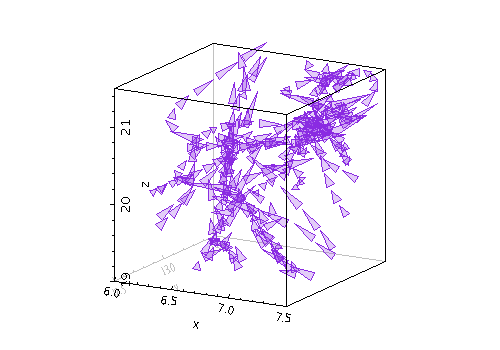
   stilts plot2cube in=gavo_g2.fits
                    x=x y=y z=z xdelta=velX ydelta=velY zdelta=velZ autoscale=true
                    color=BlueViolet scale=1.5
                    layer1=xyzvector shading1=transparent opaque1=5 arrow1=medium_filled_dart
                    layer2=xyzvector shading2=flat arrow2=medium_open_dart
                    xmin=6 xmax=7.5 ymin=12.5 ymax=13.5 zmin=19 zmax=21.5
arrowN = small_arrow|medium_arrow|... (MultiPointShape)
The available options are:
small_arrow
medium_arrow
large_arrow
small_open_dart
medium_open_dart
large_open_dart
small_filled_dart
medium_filled_dart
large_filled_dart
lines
capped_lines
[Default: small_arrow]
autoscaleN = true|false (Boolean)
If auto-scaling is on, then markers will keep approximately the same screen size during zoom operations; if it's off, they will keep the same size in data coordinates.
Marker size is also affected by the
scale parameter.
[Default: false]
icmdN = <cmds> (ProcessingStep[])
inN.
The value of this parameter is one or more of the filter
commands described in Section 6.1.
If more than one is given, they must be separated by
semicolon characters (";").
This parameter can be repeated multiple times on the same
command line to build up a list of processing steps.
The sequence of commands given in this way
defines the processing pipeline which is performed on the table.
Commands may alternatively be supplied in an external file,
by using the indirection character '@'.
Thus a value of "@filename"
causes the file filename to be read for a list
of filter commands to execute. The commands in the file
may be separated by newline characters and/or semicolons,
and lines which are blank or which start with a
'#' character are ignored.
A backslash character '\' at the end of a line
joins it with the following line.
ifmtN = <in-format> (String)
inN.
The known formats are listed in Section 5.1.1.
This flag can be used if you know what format your
table is in.
If it has the special value
(auto) (the default),
then an attempt will be
made to detect the format of the table automatically.
This cannot always be done correctly however, in which case
the program will exit with an error explaining which
formats were attempted.
This parameter is ignored for scheme-specified tables.
[Default: (auto)]
inN = <table> (StarTable)
-",
meaning standard input.
In this case the input format must be given explicitly
using the ifmtN
parameter.
Note that not all formats can be streamed in this way.:<scheme-name>:<scheme-args>.<" character at the start,
or a "|" character at the end
("<syscmd" or
"syscmd|").
This executes the given pipeline and reads from its
standard output.
This will probably only work on unix-like systems.istreamN = true|false (Boolean)
inN parameter
will be read as a stream.
It is necessary to give the
ifmtN parameter
in this case.
Depending on the required operations and processing mode,
this may cause the read to fail (sometimes it is necessary
to read the table more than once).
It is not normally necessary to set this flag;
in most cases the data will be streamed automatically
if that is the best thing to do.
However it can sometimes result in less resource usage when
processing large files in certain formats (such as VOTable).
This parameter is ignored for scheme-specified tables.
[Default: false]
scaleN = <factor> (Double)
[Default: 1]
shadingN = flat|translucent|transparent|density|aux|weighted|paux|pweighted <shade-paramsN> (ShapeMode)
[Default: flat]
thickN = <int-value> (Integer)
[Default: 0]
xN = <num-expr> (String)
The value is a numeric algebraic expression based on column names as described in Section 10.
xdeltaN = <num-expr> (String)
The value is a numeric algebraic expression based on column names as described in Section 10.
yN = <num-expr> (String)
The value is a numeric algebraic expression based on column names as described in Section 10.
ydeltaN = <num-expr> (String)
The value is a numeric algebraic expression based on column names as described in Section 10.
zN = <num-expr> (String)
The value is a numeric algebraic expression based on column names as described in Section 10.
zdeltaN = <num-expr> (String)
The value is a numeric algebraic expression based on column names as described in Section 10.
xyzerror
Plots symmetric or asymmetric error bars in some or all of the plot dimensions. The shape of the error "bars" is quite configurable, including (for 2-d and 3-d errors) ellipses, rectangles etc aligned with the axes.
Usage Overview:
   layerN=xyzerror errorbarN=none|lines|capped_lines|... thickN=<int-value>
                   shadingN=flat|translucent|transparent|density|aux|weighted|paux|pweighted <shade-paramsN>
                   xN=<num-expr> yN=<num-expr> zN=<num-expr> xerrhiN=<num-expr>
                   xerrloN=<num-expr> yerrhiN=<num-expr> yerrloN=<num-expr>
                   zerrhiN=<num-expr> zerrloN=<num-expr> inN=<table>
                   ifmtN=<in-format> istreamN=true|false icmdN=<cmds>
All the parameters listed here
affect only the relevant layer,
identified by the suffix
N.
Example:
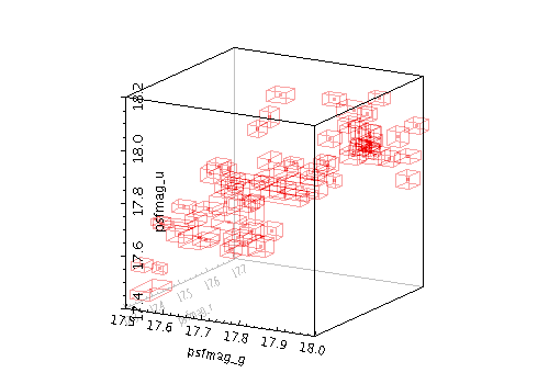
   stilts plot2cube in=dr5qso.fits icmd='select morphology==1'
                    x=psfmag_g xerrhi=psfmagerr_g
                    y=psfmag_r yerrhi=psfmagerr_r
                    z=psfmag_u zerrhi=psfmagerr_u
                    layer1=mark
                    layer2=xyzerror errorbar2=cuboid
                    shading=transparent opaque=3
                    xmin=17.5 xmax=18 ymin=17.3 ymax=17.7 zmin=17.4 zmax=18.2
errorbarN = none|lines|capped_lines|... (MultiPointShape)
The available options are:
none
lines
capped_lines
caps
arrows
cuboid
ellipse
crosshair_ellipse
rectangle
crosshair_rectangle
filled_ellipse
filled_rectangle
[Default: lines]
icmdN = <cmds> (ProcessingStep[])
inN.
The value of this parameter is one or more of the filter
commands described in Section 6.1.
If more than one is given, they must be separated by
semicolon characters (";").
This parameter can be repeated multiple times on the same
command line to build up a list of processing steps.
The sequence of commands given in this way
defines the processing pipeline which is performed on the table.
Commands may alternatively be supplied in an external file,
by using the indirection character '@'.
Thus a value of "@filename"
causes the file filename to be read for a list
of filter commands to execute. The commands in the file
may be separated by newline characters and/or semicolons,
and lines which are blank or which start with a
'#' character are ignored.
A backslash character '\' at the end of a line
joins it with the following line.
ifmtN = <in-format> (String)
inN.
The known formats are listed in Section 5.1.1.
This flag can be used if you know what format your
table is in.
If it has the special value
(auto) (the default),
then an attempt will be
made to detect the format of the table automatically.
This cannot always be done correctly however, in which case
the program will exit with an error explaining which
formats were attempted.
This parameter is ignored for scheme-specified tables.
[Default: (auto)]
inN = <table> (StarTable)
-",
meaning standard input.
In this case the input format must be given explicitly
using the ifmtN
parameter.
Note that not all formats can be streamed in this way.:<scheme-name>:<scheme-args>.<" character at the start,
or a "|" character at the end
("<syscmd" or
"syscmd|").
This executes the given pipeline and reads from its
standard output.
This will probably only work on unix-like systems.istreamN = true|false (Boolean)
inN parameter
will be read as a stream.
It is necessary to give the
ifmtN parameter
in this case.
Depending on the required operations and processing mode,
this may cause the read to fail (sometimes it is necessary
to read the table more than once).
It is not normally necessary to set this flag;
in most cases the data will be streamed automatically
if that is the best thing to do.
However it can sometimes result in less resource usage when
processing large files in certain formats (such as VOTable).
This parameter is ignored for scheme-specified tables.
[Default: false]
shadingN = flat|translucent|transparent|density|aux|weighted|paux|pweighted <shade-paramsN> (ShapeMode)
[Default: flat]
thickN = <int-value> (Integer)
[Default: 0]
xN = <num-expr> (String)
The value is a numeric algebraic expression based on column names as described in Section 10.
xerrhiN = <num-expr> (String)
The value is a numeric algebraic expression based on column names as described in Section 10.
xerrloN = <num-expr> (String)
The value is a numeric algebraic expression based on column names as described in Section 10.
yN = <num-expr> (String)
The value is a numeric algebraic expression based on column names as described in Section 10.
yerrhiN = <num-expr> (String)
The value is a numeric algebraic expression based on column names as described in Section 10.
yerrloN = <num-expr> (String)
The value is a numeric algebraic expression based on column names as described in Section 10.
zN = <num-expr> (String)
The value is a numeric algebraic expression based on column names as described in Section 10.
zerrhiN = <num-expr> (String)
The value is a numeric algebraic expression based on column names as described in Section 10.
zerrloN = <num-expr> (String)
The value is a numeric algebraic expression based on column names as described in Section 10.
line3d
Plots a point-to-point line joining
up the positions of data points in three dimensions.
There are additional options to pre-sort the points
by a given quantity before drawing the lines
(using the sort value),
and to vary the colour of the line along its length
(using the aux value).
The options for controlling the Aux colour map
are controlled at the level of the plot itself,
rather than by per-layer configuration.
Note that the line positioning in 3d and the line segment aux colouring is somewhat approximate. In most cases it is good enough for visual inspection, but pixel-level examination may reveal discrepancies.
Usage Overview:
   layerN=line3d colorN=<rrggbb>|red|blue|... thickN=<pixels>
                 <pos-coord-paramsN> auxN=<num-expr> sortN=<num-expr>
                 inN=<table> ifmtN=<in-format> istreamN=true|false icmdN=<cmds>
All the parameters listed here
affect only the relevant layer,
identified by the suffix
N.
<pos-coord-paramsN>
give a position for each row of the input table.
Their form depends on the plot geometry,
i.e. which plotting command is used.
For a plane plot (plot2plane)
the parameters would be
xN and yN.
The coordinate parameter values are in all cases strings
interpreted as numeric expressions based on column names.
These can be column names, fixed values or algebraic
expressions as described in Section 10.
Example:
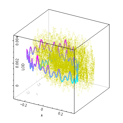
   stilts plot2cube in=iers.fits x=x y=y z=LOD
                    layer1=line3d icmd1='select decYear>1963&&decYear<1964.5' thick1=3 aux1=LOD
                    layer2=mark shading2=translucent color2=cccc00 translevel2=0.35
                    auxmap=cyan-magenta auxvisible=false legend=false
                    phi=-150 theta=25 psi=180 xpix=400 ypix=400
auxN = <num-expr> (String)
The value is a numeric algebraic expression based on column names as described in Section 10.
colorN = <rrggbb>|red|blue|... (Color)
The standard plotting colour names are
red, blue, green, grey, magenta, cyan, orange, pink, yellow, black, light_grey, white.
However, many other common colour names (too many to list here)
are also understood.
The list currently contains those colour names understood
by most web browsers,
from AliceBlue to YellowGreen,
listed e.g. in the
Extended color keywords section of
the CSS3 standard.
Alternatively, a six-digit hexadecimal number RRGGBB
may be supplied,
optionally prefixed by "#" or "0x",
giving red, green and blue intensities,
e.g. "ff00ff", "#ff00ff"
or "0xff00ff" for magenta.
[Default: red]
icmdN = <cmds> (ProcessingStep[])
inN.
The value of this parameter is one or more of the filter
commands described in Section 6.1.
If more than one is given, they must be separated by
semicolon characters (";").
This parameter can be repeated multiple times on the same
command line to build up a list of processing steps.
The sequence of commands given in this way
defines the processing pipeline which is performed on the table.
Commands may alternatively be supplied in an external file,
by using the indirection character '@'.
Thus a value of "@filename"
causes the file filename to be read for a list
of filter commands to execute. The commands in the file
may be separated by newline characters and/or semicolons,
and lines which are blank or which start with a
'#' character are ignored.
A backslash character '\' at the end of a line
joins it with the following line.
ifmtN = <in-format> (String)
inN.
The known formats are listed in Section 5.1.1.
This flag can be used if you know what format your
table is in.
If it has the special value
(auto) (the default),
then an attempt will be
made to detect the format of the table automatically.
This cannot always be done correctly however, in which case
the program will exit with an error explaining which
formats were attempted.
This parameter is ignored for scheme-specified tables.
[Default: (auto)]
inN = <table> (StarTable)
-",
meaning standard input.
In this case the input format must be given explicitly
using the ifmtN
parameter.
Note that not all formats can be streamed in this way.:<scheme-name>:<scheme-args>.<" character at the start,
or a "|" character at the end
("<syscmd" or
"syscmd|").
This executes the given pipeline and reads from its
standard output.
This will probably only work on unix-like systems.istreamN = true|false (Boolean)
inN parameter
will be read as a stream.
It is necessary to give the
ifmtN parameter
in this case.
Depending on the required operations and processing mode,
this may cause the read to fail (sometimes it is necessary
to read the table more than once).
It is not normally necessary to set this flag;
in most cases the data will be streamed automatically
if that is the best thing to do.
However it can sometimes result in less resource usage when
processing large files in certain formats (such as VOTable).
This parameter is ignored for scheme-specified tables.
[Default: false]
sortN = <num-expr> (String)
Note that if the required order is in fact the natural order of the table, it is better to leave this value blank, since sorting is a potentially expensive step.
The value is a numeric algebraic expression based on column names as described in Section 10.
thickN = <pixels> (Integer)
[Default: 1]
spheregrid
Plots a spherical grid around the origin of a 3-d plot. The radius of the sphere can be configured explicitly, otherwise a suitable default value (that should make at least some of the grid visible) will be chosen.
Usage Overview:
   layerN=spheregrid radiusN=<number> gridcolorN=<rrggbb>|red|blue|...
                     thickN=<pixels> nlonN=<int-value> nlatN=<int-value>
All the parameters listed here
affect only the relevant layer,
identified by the suffix
N.
Example:
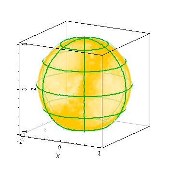
   stilts plot2sphere legend=false xpix=350 ypix=350
                      layer1=mark in1=tgas_source.fits lon1=ra lat1=dec r1=1
                      shading1=transparent opaque1=850 color1=orange
                      layer2=spheregrid gridcolor2=green thick2=2
gridcolorN = <rrggbb>|red|blue|... (Color)
The standard plotting colour names are
red, blue, green, grey, magenta, cyan, orange, pink, yellow, black, light_grey, white.
However, many other common colour names (too many to list here)
are also understood.
The list currently contains those colour names understood
by most web browsers,
from AliceBlue to YellowGreen,
listed e.g. in the
Extended color keywords section of
the CSS3 standard.
Alternatively, a six-digit hexadecimal number RRGGBB
may be supplied,
optionally prefixed by "#" or "0x",
giving red, green and blue intensities,
e.g. "ff00ff", "#ff00ff"
or "0xff00ff" for magenta.
[Default: grey]
nlatN = <int-value> (Integer)
[Default: 2]
nlonN = <int-value> (Integer)
[Default: 3]
radiusN = <number> (Double)
[Default: -1]
thickN = <pixels> (Integer)
[Default: 1]
yerror
Plots symmetric or asymmetric error bars in the Y direction.
Usage Overview:
   layerN=yerror errorbarN=none|lines|capped_lines|caps|arrows
                 thickN=<int-value> shadingN=flat <shade-paramsN>
                 tN=<time-expr> ttypeN=DecYear|MJD|JD|Unix|Iso8601
                 yN=<num-expr> yerrhiN=<num-expr> yerrloN=<num-expr>
                 inN=<table> ifmtN=<in-format> istreamN=true|false icmdN=<cmds>
All the parameters listed here
affect only the relevant layer,
identified by the suffix
N.
Example:
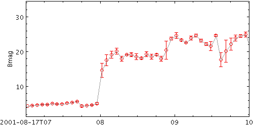
   stilts plot2time in=ACE_data.vot t=epoch y=Bmag
                    layer1=yerror yerrhi1=sigma_B errorbar1=capped_lines
                    layer2=mark shape2=open_circle size2=3
                    layer3=line color3=a0a0a0
                    tmin=2001-08-17T07 tmax=2001-08-17T10 ypix=250
errorbarN = none|lines|capped_lines|caps|arrows (MultiPointShape)
The available options are:
none
lines
capped_lines
caps
arrows
[Default: lines]
icmdN = <cmds> (ProcessingStep[])
inN.
The value of this parameter is one or more of the filter
commands described in Section 6.1.
If more than one is given, they must be separated by
semicolon characters (";").
This parameter can be repeated multiple times on the same
command line to build up a list of processing steps.
The sequence of commands given in this way
defines the processing pipeline which is performed on the table.
Commands may alternatively be supplied in an external file,
by using the indirection character '@'.
Thus a value of "@filename"
causes the file filename to be read for a list
of filter commands to execute. The commands in the file
may be separated by newline characters and/or semicolons,
and lines which are blank or which start with a
'#' character are ignored.
A backslash character '\' at the end of a line
joins it with the following line.
ifmtN = <in-format> (String)
inN.
The known formats are listed in Section 5.1.1.
This flag can be used if you know what format your
table is in.
If it has the special value
(auto) (the default),
then an attempt will be
made to detect the format of the table automatically.
This cannot always be done correctly however, in which case
the program will exit with an error explaining which
formats were attempted.
This parameter is ignored for scheme-specified tables.
[Default: (auto)]
inN = <table> (StarTable)
-",
meaning standard input.
In this case the input format must be given explicitly
using the ifmtN
parameter.
Note that not all formats can be streamed in this way.:<scheme-name>:<scheme-args>.<" character at the start,
or a "|" character at the end
("<syscmd" or
"syscmd|").
This executes the given pipeline and reads from its
standard output.
This will probably only work on unix-like systems.istreamN = true|false (Boolean)
inN parameter
will be read as a stream.
It is necessary to give the
ifmtN parameter
in this case.
Depending on the required operations and processing mode,
this may cause the read to fail (sometimes it is necessary
to read the table more than once).
It is not normally necessary to set this flag;
in most cases the data will be streamed automatically
if that is the best thing to do.
However it can sometimes result in less resource usage when
processing large files in certain formats (such as VOTable).
This parameter is ignored for scheme-specified tables.
[Default: false]
shadingN = flat <shade-paramsN> (ShapeMode)
[Default: flat]
tN = <time-expr> (String)
The value is a Time value algebraic expression based on column names as described in Section 10.
thickN = <int-value> (Integer)
[Default: 0]
ttypeN = DecYear|MJD|JD|Unix|Iso8601 (TimeMapper)
tN is supplied.
Options are:
DecYear: Years since 0 ADMJD: Modified Julian DateJD: Julian DayUnix: Seconds since midnight 1 Jan 1970Iso8601: ISO 8601 stringtN value.
yN = <num-expr> (String)
The value is a numeric algebraic expression based on column names as described in Section 10.
yerrhiN = <num-expr> (String)
The value is a numeric algebraic expression based on column names as described in Section 10.
yerrloN = <num-expr> (String)
The value is a numeric algebraic expression based on column names as described in Section 10.
spectrogram
Plots spectrograms. A spectrogram is a sequence of spectra plotted as vertical 1-d images, each one plotted at a different horizontal coordinate.
This specialised layer is only available for
time plots.
The way that data values are mapped to colours is usually controlled by options at the level of the plot itself, rather than by per-layer configuration.
Usage Overview:
   layerN=spectrogram scalespecN=true|false tN=<time-expr>
                      ttypeN=DecYear|MJD|JD|Unix|Iso8601 spectrumN=<array-expr>
                      twidthN=<num-expr> inN=<table> ifmtN=<in-format>
                      istreamN=true|false icmdN=<cmds>
All the parameters listed here
affect only the relevant layer,
identified by the suffix
N.
Example:
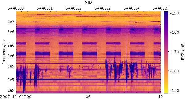
   stilts plot2time layer1=spectrogram in1=LRS_NPW_V010_20071101.cdf t1=epoch spectrum1=RX2
                    t2func=mjd t2label=MJD
                    auxfunc=linear auxmap=plasma auxclip=0,1
                    xpix=600 ypix=320
                    tmin=2007-11-01T00 tmax=2007-11-01T12
                    yscale=log ylabel=Frequency/Hz ymin=8e4 ymax=2e7
icmdN = <cmds> (ProcessingStep[])
inN.
The value of this parameter is one or more of the filter
commands described in Section 6.1.
If more than one is given, they must be separated by
semicolon characters (";").
This parameter can be repeated multiple times on the same
command line to build up a list of processing steps.
The sequence of commands given in this way
defines the processing pipeline which is performed on the table.
Commands may alternatively be supplied in an external file,
by using the indirection character '@'.
Thus a value of "@filename"
causes the file filename to be read for a list
of filter commands to execute. The commands in the file
may be separated by newline characters and/or semicolons,
and lines which are blank or which start with a
'#' character are ignored.
A backslash character '\' at the end of a line
joins it with the following line.
ifmtN = <in-format> (String)
inN.
The known formats are listed in Section 5.1.1.
This flag can be used if you know what format your
table is in.
If it has the special value
(auto) (the default),
then an attempt will be
made to detect the format of the table automatically.
This cannot always be done correctly however, in which case
the program will exit with an error explaining which
formats were attempted.
This parameter is ignored for scheme-specified tables.
[Default: (auto)]
inN = <table> (StarTable)
-",
meaning standard input.
In this case the input format must be given explicitly
using the ifmtN
parameter.
Note that not all formats can be streamed in this way.:<scheme-name>:<scheme-args>.<" character at the start,
or a "|" character at the end
("<syscmd" or
"syscmd|").
This executes the given pipeline and reads from its
standard output.
This will probably only work on unix-like systems.istreamN = true|false (Boolean)
inN parameter
will be read as a stream.
It is necessary to give the
ifmtN parameter
in this case.
Depending on the required operations and processing mode,
this may cause the read to fail (sometimes it is necessary
to read the table more than once).
It is not normally necessary to set this flag;
in most cases the data will be streamed automatically
if that is the best thing to do.
However it can sometimes result in less resource usage when
processing large files in certain formats (such as VOTable).
This parameter is ignored for scheme-specified tables.
[Default: false]
scalespecN = true|false (Boolean)
If this flag is set false, or if no suitable array can be found, the vertical axis just represents channel indices and so is labelled from 0 to the number of channels per spectrum.
This configuration item is somewhat experimental; the details of how the spectral axis is configured may change in future releases.
[Default: true]
spectrumN = <array-expr> (String)
The value is an array-valued algebraic expression based on column names as described in Section 10. Some of the functions in the Arrays class may be useful here.
tN = <time-expr> (String)
The value is a Time value algebraic expression based on column names as described in Section 10.
ttypeN = DecYear|MJD|JD|Unix|Iso8601 (TimeMapper)
tN is supplied.
Options are:
DecYear: Years since 0 ADMJD: Modified Julian DateJD: Julian DayUnix: Seconds since midnight 1 Jan 1970Iso8601: ISO 8601 stringtN value.
twidthN = <num-expr> (String)
The value is a numeric algebraic expression based on column names as described in Section 10.
Some plot layer types
have an associated shading parameter
which determines how plotted markers are coloured.
This is independent of the marker shapes
(which may be points, vectors, ellipses, ...)
but may be affected by how many markers are plotted on top of each other,
additional input table values, selected colour maps etc.
For the simplest shading types
(e.g. flat)
it's just a case of choosing a colour,
but the more complex ones have several associated parameters.
The various shading types and their usages are described in the following subsections.
auto
Paints isolated points in their selected colour but where multiple points in the same layer overlap it adjusts the clour by darkening it. This means that for isolated points (most or all points in a non-crowded plot, or outliers in a crowded plot) it behaves just like flat mode, but it's easy to see where overdense regions lie.
This is like density mode, but with no user-configurable options.
Usage:
shadingN=auto colorN=<rrggbb>|red|blue|...
All the parameters listed here
affect only the relevant layer,
identified by the suffix
N.
Example:
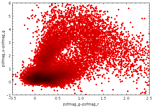
   stilts plot2plane layer1=mark in1=dr5qso.fits
                     x1=psfmag_g-psfmag_r y1=psfmag_u-psfmag_g size1=2
                     shading1=auto
                     xmin=-0.5 xmax=2.5 ymin=-1 ymax=6
Associated parameters are as follows:
colorN = <rrggbb>|red|blue|... (Color)
The standard plotting colour names are
red, blue, green, grey, magenta, cyan, orange, pink, yellow, black, light_grey, white.
However, many other common colour names (too many to list here)
are also understood.
The list currently contains those colour names understood
by most web browsers,
from AliceBlue to YellowGreen,
listed e.g. in the
Extended color keywords section of
the CSS3 standard.
Alternatively, a six-digit hexadecimal number RRGGBB
may be supplied,
optionally prefixed by "#" or "0x",
giving red, green and blue intensities,
e.g. "ff00ff", "#ff00ff"
or "0xff00ff" for magenta.
[Default: red]
flat
Paints markers in a single fixed colour.
Usage:
shadingN=flat colorN=<rrggbb>|red|blue|...
All the parameters listed here
affect only the relevant layer,
identified by the suffix
N.
Example:
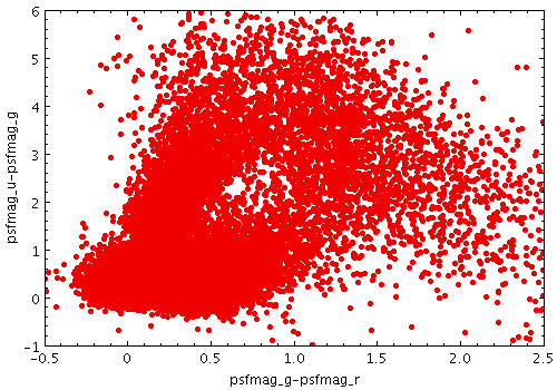
   stilts plot2plane layer1=mark in1=dr5qso.fits
                     x1=psfmag_g-psfmag_r y1=psfmag_u-psfmag_g size1=2
                     shading1=flat
                     xmin=-0.5 xmax=2.5 ymin=-1 ymax=6
Associated parameters are as follows:
colorN = <rrggbb>|red|blue|... (Color)
The standard plotting colour names are
red, blue, green, grey, magenta, cyan, orange, pink, yellow, black, light_grey, white.
However, many other common colour names (too many to list here)
are also understood.
The list currently contains those colour names understood
by most web browsers,
from AliceBlue to YellowGreen,
listed e.g. in the
Extended color keywords section of
the CSS3 standard.
Alternatively, a six-digit hexadecimal number RRGGBB
may be supplied,
optionally prefixed by "#" or "0x",
giving red, green and blue intensities,
e.g. "ff00ff", "#ff00ff"
or "0xff00ff" for magenta.
[Default: red]
translucent
Paints markers in a transparent version of their selected colour. The degree of transparency is determined by how many points are plotted on top of each other and by the transparency level. Unlike transparent mode, the transparency varies according to the average point density in the plot, so leaving the setting the same as you zoom in and out usually has a sensible effect.
Usage:
shadingN=translucent colorN=<rrggbb>|red|blue|... translevelN=<number>
All the parameters listed here
affect only the relevant layer,
identified by the suffix
N.
Example:
   stilts plot2plane layer1=mark in1=dr5qso.fits
                     x1=psfmag_g-psfmag_r y1=psfmag_u-psfmag_g size1=2
                     shading1=translucent
                     xmin=-0.5 xmax=2.5 ymin=-1 ymax=6
Associated parameters are as follows:
colorN = <rrggbb>|red|blue|... (Color)
The standard plotting colour names are
red, blue, green, grey, magenta, cyan, orange, pink, yellow, black, light_grey, white.
However, many other common colour names (too many to list here)
are also understood.
The list currently contains those colour names understood
by most web browsers,
from AliceBlue to YellowGreen,
listed e.g. in the
Extended color keywords section of
the CSS3 standard.
Alternatively, a six-digit hexadecimal number RRGGBB
may be supplied,
optionally prefixed by "#" or "0x",
giving red, green and blue intensities,
e.g. "ff00ff", "#ff00ff"
or "0xff00ff" for magenta.
[Default: red]
translevelN = <number> (Double)
[Default: 0.1]
transparent
Paints markers in a transparent version of their selected colour. The degree of transparency is determined by how many points are plotted on top of each other and by the opaque limit. The opaque limit fixes how many points must be plotted on top of each other to completely obscure the background. This is set to a fixed value, so a transparent level that works well for a crowded region (or low magnification) may not work so well for a sparse region (or when zoomed in).
Usage:
shadingN=transparent colorN=<rrggbb>|red|blue|... opaqueN=<number>
All the parameters listed here
affect only the relevant layer,
identified by the suffix
N.
Example:
   stilts plot2plane layer1=mark in1=dr5qso.fits
                     x1=psfmag_g-psfmag_r y1=psfmag_u-psfmag_g size1=2
                     shading1=transparent
                     xmin=-0.5 xmax=2.5 ymin=-1 ymax=6
Associated parameters are as follows:
colorN = <rrggbb>|red|blue|... (Color)
The standard plotting colour names are
red, blue, green, grey, magenta, cyan, orange, pink, yellow, black, light_grey, white.
However, many other common colour names (too many to list here)
are also understood.
The list currently contains those colour names understood
by most web browsers,
from AliceBlue to YellowGreen,
listed e.g. in the
Extended color keywords section of
the CSS3 standard.
Alternatively, a six-digit hexadecimal number RRGGBB
may be supplied,
optionally prefixed by "#" or "0x",
giving red, green and blue intensities,
e.g. "ff00ff", "#ff00ff"
or "0xff00ff" for magenta.
[Default: red]
opaqueN = <number> (Double)
[Default: 4]
density
Paints markers using a configurable colour map to indicate how many points are plotted over each other. Specifically, it colours each pixel according to how many times that pixel has has been covered by one of the markers plotted by the layer in question. To put it another way, it generates a false-colour density map with pixel granularity using a smoothing kernel of the form of the markers plotted by the layer. The upshot is that you can see the plot density of points or other markers plotted.
This is like auto mode, but with more user-configurable options.
Usage:
   shadingN=density colorN=<rrggbb>|red|blue|...
                    densemapN=<map-name>|<color>-<color>[-<color>...]
                    denseclipN=<lo>,<hi> denseflipN=true|false
                    densequantN=<number> densesubN=<lo>,<hi>
                    densefuncN=log|linear|histogram|...
All the parameters listed here
affect only the relevant layer,
identified by the suffix
N.
Example:
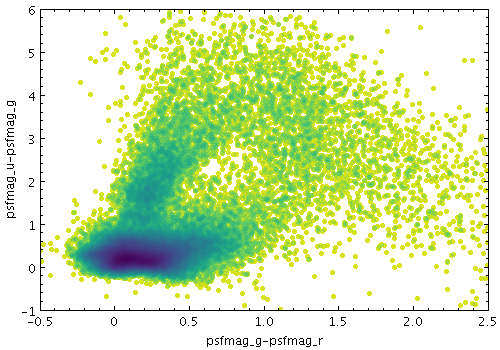
   stilts plot2plane layer1=mark in1=dr5qso.fits
                     x1=psfmag_g-psfmag_r y1=psfmag_u-psfmag_g size1=2
                     shading1=density densemap1=viridis
                     xmin=-0.5 xmax=2.5 ymin=-1 ymax=6
Associated parameters are as follows:
colorN = <rrggbb>|red|blue|... (Color)
The standard plotting colour names are
red, blue, green, grey, magenta, cyan, orange, pink, yellow, black, light_grey, white.
However, many other common colour names (too many to list here)
are also understood.
The list currently contains those colour names understood
by most web browsers,
from AliceBlue to YellowGreen,
listed e.g. in the
Extended color keywords section of
the CSS3 standard.
Alternatively, a six-digit hexadecimal number RRGGBB
may be supplied,
optionally prefixed by "#" or "0x",
giving red, green and blue intensities,
e.g. "ff00ff", "#ff00ff"
or "0xff00ff" for magenta.
[Default: red]
denseclipN = <lo>,<hi> (Subrange)
If the full range 0,1 is used,
the whole range of colours specified by the selected
shader will be used.
But if for instance a value of 0,0.5 is given,
only those colours at the left hand end of the ramp
will be seen.
If the null (default) value is chosen,
a default clip will be used.
This generally covers most or all of the range 0-1
but for colour maps which fade to white,
a small proportion of the lower end may be excluded,
to ensure that all the colours are visually distinguishable
from a white background.
This default is usually a good idea if the colour map
is being used with something like a scatter plot,
where markers are plotted against a white background.
However, for something like a density map when the whole
plotting area is tiled with colours from the map,
it may be better to supply the whole range
0,1 explicitly.
denseflipN = true|false (Boolean)
[Default: false]
densefuncN = log|linear|histogram|... (Scaling)
The available options are:
log: Logarithmic scaling, positive values onlylinear: Linear scalinghistogram: Scaling follows data distribution, with linear axishistolog: Scaling follows data distribution, with logarithmic axis, positive values onlyasinh: Asinh scaling, wide dynamic range for both positive and negative valuessqrt: Square root scalingsquare: Square scalingacos: Inverse cosine Scalingcos: Cosine ScalingFor all these options,
the full range of valid data values is used,
and displayed on the colour bar
if applicable (though it can be restricted using the densesub option)
Note that logarithmic-based options
Log and
HistoLog
will ignore non-positive values.
The Linear,
Log,
Square and
Sqrt options
just apply the named function to the full data range.
The histogram options on the other hand use a scaling function
that corresponds to the actual distribution of the data, so that
there are about the same number of points (or pixels, or whatever
is being scaled) of each colour.
The histogram options are somewhat more expensive,
but can be a good choice if you are exploring data whose
distribution is unknown or not well-behaved over
its min-max range.
The Histogram and
HistoLog options both
assign the colours in the same way, but they display the colour
ramp with linear or logarithmic annotation respectively;
the HistoLog option also ignores
non-positive values.
[Default: log]
densemapN = <map-name>|<color>-<color>[-<color>...] (Shader)
A mixed bag of colour ramps are available
as listed in Section 8.7:
blacker,
whiter,
inferno,
magma,
plasma,
viridis,
cividis,
cubehelix,
sron,
rainbow,
rainbow2,
rainbow3,
pastel,
cosmic,
ember,
gothic,
rainforest,
voltage,
bubblegum,
gem,
chroma,
sunset,
neon,
tropical,
accent,
gnuplot,
gnuplot2,
specxby,
set1,
paired,
hotcold,
guppy,
iceburn,
redshift,
pride,
rdbu,
piyg,
brbg,
cyan-magenta,
red-blue,
brg,
heat,
cold,
light,
greyscale,
colour,
standard,
bugn,
bupu,
orrd,
pubu,
purd,
painbow,
huecl,
infinity,
hue,
intensity,
rgb_red,
rgb_green,
rgb_blue,
hsv_h,
hsv_s,
hsv_v,
yuv_y,
yuv_u,
yuv_v,
scale_hsv_s,
scale_hsv_v,
scale_yuv_y.
Note:
many of these, including rainbow-like ones,
are frowned upon by the visualisation community.
You can also construct your own custom colour map
by giving a sequence of colour names separated by
minus sign ("-") characters.
In this case the ramp is a linear interpolation
between each pair of colours named,
using the same syntax as when specifying
a colour value.
So for instance
"yellow-hotpink-#0000ff"
would shade from yellow via hot pink to blue.
[Default: blacker]
densequantN = <number> (Double)
If left blank, the colour map is nominally continuous (though in practice it may be quantised to a medium-sized number like 256).
densesubN = <lo>,<hi> (Subrange)
The default value "0,1" therefore has
no effect.
The range could be restricted to its lower half
with the value 0,0.5.
[Default: 0,1]
aux
Paints markers in a colour determined by the value of an additional data coordinate, using a colour map shared between all similar layers. The marker colours then represent an additional dimension of the plot. You can also adjust the transparency of the colours used. The way that data values are mapped to colours is usually controlled by options at the level of the plot itself, rather than by per-layer configuration.
Usage:
   shadingN=aux auxN=<num-expr> auxnullcolorN=<rrggbb>|red|blue|...
                opaqueN=<number>
All the parameters listed here
affect only the relevant layer,
identified by the suffix
N.
Example:
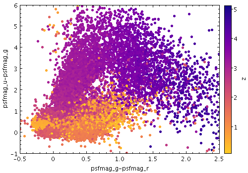
   stilts plot2plane layer1=mark in1=dr5qso.fits
                     x1=psfmag_g-psfmag_r y1=psfmag_u-psfmag_g size1=2
                     shading1=aux aux1=z auxmap=plasma
                     xmin=-0.5 xmax=2.5 ymin=-1 ymax=6
Associated parameters are as follows:
auxN = <num-expr> (String)
This parameter gives a column name, fixed value, or algebraic expression for the
aux coordinate
for layer N.
The value is a numeric algebraic expression based on column names
as described in Section 10.
auxnullcolorN = <rrggbb>|red|blue|... (Color)
The standard plotting colour names are
red, blue, green, grey, magenta, cyan, orange, pink, yellow, black, light_grey, white.
However, many other common colour names (too many to list here)
are also understood.
The list currently contains those colour names understood
by most web browsers,
from AliceBlue to YellowGreen,
listed e.g. in the
Extended color keywords section of
the CSS3 standard.
Alternatively, a six-digit hexadecimal number RRGGBB
may be supplied,
optionally prefixed by "#" or "0x",
giving red, green and blue intensities,
e.g. "ff00ff", "#ff00ff"
or "0xff00ff" for magenta.
If the value is null, then points with a null Aux value will not be plotted at all.
[Default: grey]
opaqueN = <number> (Double)
[Default: 1]
weighted
Paints markers like the Density mode, but with optional weighting by an additional coordinate; the colour map is shared between layers. You can configure how the weighted coordinates are combined to give the final weighted result. The way that data values are mapped to colours is usually controlled by options at the level of the plot itself, rather than by per-layer configuration.
Usage:
   shadingN=weighted weightN=<num-expr> colorN=<rrggbb>|red|blue|...
                     combineN=sum|count|mean|median|...
All the parameters listed here
affect only the relevant layer,
identified by the suffix
N.
Example:
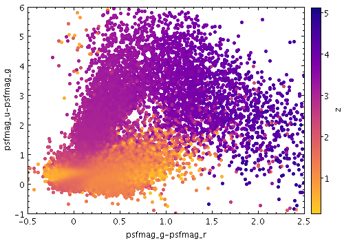
   stilts plot2plane layer1=mark in1=dr5qso.fits
                     x1=psfmag_g-psfmag_r y1=psfmag_u-psfmag_g size1=2
                     shading1=weighted weight1=z auxmap=plasma
                     xmin=-0.5 xmax=2.5 ymin=-1 ymax=6
Associated parameters are as follows:
colorN = <rrggbb>|red|blue|... (Color)
The standard plotting colour names are
red, blue, green, grey, magenta, cyan, orange, pink, yellow, black, light_grey, white.
However, many other common colour names (too many to list here)
are also understood.
The list currently contains those colour names understood
by most web browsers,
from AliceBlue to YellowGreen,
listed e.g. in the
Extended color keywords section of
the CSS3 standard.
Alternatively, a six-digit hexadecimal number RRGGBB
may be supplied,
optionally prefixed by "#" or "0x",
giving red, green and blue intensities,
e.g. "ff00ff", "#ff00ff"
or "0xff00ff" for magenta.
[Default: red]
combineN = sum|count|mean|median|... (Combiner)
When a weight is in use,
mean or
sum
are typically sensible choices.
If there is no weight (a pure density map)
then count is usually better,
but in that case it may make more sense
(it is more efficient)
to use one of the other shading modes instead.
The available options are:
sum: the sum of all the combined values per bincount: the number of non-blank values per bin (weight is ignored)mean: the mean of the combined valuesmedian: the medianq1: first quartileq3: third quartilemin: the minimum of all the combined valuesmax: the maximum of all the combined valuesstdev: the sample standard deviation of the combined valuesstdev_pop: the population standard deviation of the combined valueshit: 1 if any values present, NaN otherwise (weight is ignored)[Default: mean]
weightN = <num-expr> (String)
This parameter gives a column name, fixed value, or algebraic expression for the
weight coordinate
for layer N.
The value is a numeric algebraic expression based on column names
as described in Section 10.
paux
Paints markers in a colour determined by the value of an additional data coordinate, using a colour map private to this layer. The marker colours then represent an additional dimension of the plot. You can also adjust the transparency of the colours used. There are additional options to adjust the way data values are mapped to colours.
This resembles
aux
mode, but the colour map is not shared with other
layers, and the colour ramp is not displayed.
So by using this mode alongside
aux or
weighted
you can make a plot that uses multiple
different colour maps,
though only one can have
an associated visible ramp.
Usage:
   shadingN=paux auxN=<num-expr> pmapN=<map-name>|<color>-<color>[-<color>...]
                 pclipN=<lo>,<hi> pflipN=true|false pquantN=<number>
                 psubN=<lo>,<hi> pfuncN=log|linear|histogram|...
                 pnullcolorN=<rrggbb>|red|blue|... opaqueN=<number>
All the parameters listed here
affect only the relevant layer,
identified by the suffix
N.
Example:
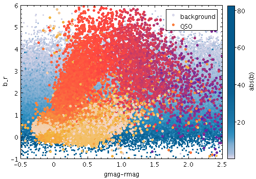
   stilts plot2plane layer1=mark in1=dr5qso.fits
                     x1=psfmag_g-psfmag_r y1=psfmag_u-psfmag_g size1=2
                     shading1=paux aux1=z pmap1=sunset
                     layer2=mark in2=:skysim:1_000_000
                     x2=gmag-rmag y2=b_r
                     shading2=weighted weight2=abs(b) auxmap=pubu auxfunc=histogram
                     leglabel1=QSO leglabel2=background legpos=.97,.97 seq=2,1
                     xmin=-0.5 xmax=2.5 ymin=-1 ymax=6
Associated parameters are as follows:
auxN = <num-expr> (String)
This parameter gives a column name, fixed value, or algebraic expression for the
aux coordinate
for layer N.
The value is a numeric algebraic expression based on column names
as described in Section 10.
opaqueN = <number> (Double)
[Default: 1]
pclipN = <lo>,<hi> (Subrange)
If the full range 0,1 is used,
the whole range of colours specified by the selected
shader will be used.
But if for instance a value of 0,0.5 is given,
only those colours at the left hand end of the ramp
will be seen.
If the null (default) value is chosen,
a default clip will be used.
This generally covers most or all of the range 0-1
but for colour maps which fade to white,
a small proportion of the lower end may be excluded,
to ensure that all the colours are visually distinguishable
from a white background.
This default is usually a good idea if the colour map
is being used with something like a scatter plot,
where markers are plotted against a white background.
However, for something like a density map when the whole
plotting area is tiled with colours from the map,
it may be better to supply the whole range
0,1 explicitly.
pflipN = true|false (Boolean)
[Default: false]
pfuncN = log|linear|histogram|... (Scaling)
The available options are:
log: Logarithmic scaling, positive values onlylinear: Linear scalinghistogram: Scaling follows data distribution, with linear axishistolog: Scaling follows data distribution, with logarithmic axis, positive values onlyasinh: Asinh scaling, wide dynamic range for both positive and negative valuessqrt: Square root scalingsquare: Square scalingacos: Inverse cosine Scalingcos: Cosine ScalingFor all these options,
the full range of valid data values is used,
and displayed on the colour bar
if applicable (though it can be restricted using the psub option)
Note that logarithmic-based options
Log and
HistoLog
will ignore non-positive values.
The Linear,
Log,
Square and
Sqrt options
just apply the named function to the full data range.
The histogram options on the other hand use a scaling function
that corresponds to the actual distribution of the data, so that
there are about the same number of points (or pixels, or whatever
is being scaled) of each colour.
The histogram options are somewhat more expensive,
but can be a good choice if you are exploring data whose
distribution is unknown or not well-behaved over
its min-max range.
The Histogram and
HistoLog options both
assign the colours in the same way, but they display the colour
ramp with linear or logarithmic annotation respectively;
the HistoLog option also ignores
non-positive values.
[Default: linear]
pmapN = <map-name>|<color>-<color>[-<color>...] (Shader)
A mixed bag of colour ramps are available
as listed in Section 8.7:
inferno,
magma,
plasma,
viridis,
cividis,
cubehelix,
sron,
rainbow,
rainbow2,
rainbow3,
pastel,
cosmic,
ember,
gothic,
rainforest,
voltage,
bubblegum,
gem,
chroma,
sunset,
neon,
tropical,
accent,
gnuplot,
gnuplot2,
specxby,
set1,
paired,
hotcold,
guppy,
iceburn,
redshift,
pride,
rdbu,
piyg,
brbg,
cyan-magenta,
red-blue,
brg,
heat,
cold,
light,
greyscale,
colour,
standard,
bugn,
bupu,
orrd,
pubu,
purd,
painbow,
huecl,
infinity,
hue,
intensity,
rgb_red,
rgb_green,
rgb_blue,
hsv_h,
hsv_s,
hsv_v,
yuv_y,
yuv_u,
yuv_v,
scale_hsv_s,
scale_hsv_v,
scale_yuv_y,
mask,
blacker,
whiter,
transparency.
Note:
many of these, including rainbow-like ones,
are frowned upon by the visualisation community.
You can also construct your own custom colour map
by giving a sequence of colour names separated by
minus sign ("-") characters.
In this case the ramp is a linear interpolation
between each pair of colours named,
using the same syntax as when specifying
a colour value.
So for instance
"yellow-hotpink-#0000ff"
would shade from yellow via hot pink to blue.
[Default: inferno]
pnullcolorN = <rrggbb>|red|blue|... (Color)
The standard plotting colour names are
red, blue, green, grey, magenta, cyan, orange, pink, yellow, black, light_grey, white.
However, many other common colour names (too many to list here)
are also understood.
The list currently contains those colour names understood
by most web browsers,
from AliceBlue to YellowGreen,
listed e.g. in the
Extended color keywords section of
the CSS3 standard.
Alternatively, a six-digit hexadecimal number RRGGBB
may be supplied,
optionally prefixed by "#" or "0x",
giving red, green and blue intensities,
e.g. "ff00ff", "#ff00ff"
or "0xff00ff" for magenta.
If the value is null, then points with a null Aux value will not be plotted at all.
[Default: grey]
pquantN = <number> (Double)
If left blank, the colour map is nominally continuous (though in practice it may be quantised to a medium-sized number like 256).
psubN = <lo>,<hi> (Subrange)
The default value "0,1" therefore has
no effect.
The range could be restricted to its lower half
with the value 0,0.5.
[Default: 0,1]
pweighted
Paints markers like the Density mode, but with optional weighting by an additional coordinate; the colour map is private to this layer. You can configure how the weighted coordinates are combined to give the final weighted result. There are additional options to adjust the way data values are mapped to colours.
This resembles
weighted mode,
but the colour map is not shared with other
layers, and the colour ramp is not displayed.
So by using this mode alongside
weighted or
aux
you can make a plot that uses multiple
different colour maps,
though only one can have
an associated visible ramp.
Usage:
   shadingN=pweighted weightN=<num-expr> colorN=<rrggbb>|red|blue|...
                      combineN=sum|count|mean|median|...
                      pmapN=<map-name>|<color>-<color>[-<color>...]
                      pclipN=<lo>,<hi> pflipN=true|false pquantN=<number>
                      psubN=<lo>,<hi> pfuncN=log|linear|histogram|...
All the parameters listed here
affect only the relevant layer,
identified by the suffix
N.
Example:
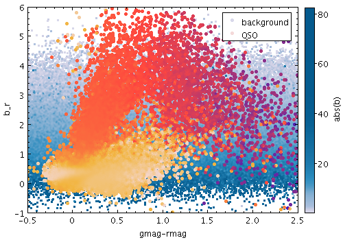
   stilts plot2plane layer1=mark in1=dr5qso.fits
                     x1=psfmag_g-psfmag_r y1=psfmag_u-psfmag_g size1=2
                     shading1=pweighted weight1=z pmap1=sunset
                     layer2=mark in2=:skysim:1_000_000
                     x2=gmag-rmag y2=b_r
                     shading2=weighted weight2=abs(b) auxmap=pubu auxfunc=histogram
                     leglabel1=QSO leglabel2=background legpos=.97,.97 seq=2,1
                     xmin=-0.5 xmax=2.5 ymin=-1 ymax=6
Associated parameters are as follows:
colorN = <rrggbb>|red|blue|... (Color)
The standard plotting colour names are
red, blue, green, grey, magenta, cyan, orange, pink, yellow, black, light_grey, white.
However, many other common colour names (too many to list here)
are also understood.
The list currently contains those colour names understood
by most web browsers,
from AliceBlue to YellowGreen,
listed e.g. in the
Extended color keywords section of
the CSS3 standard.
Alternatively, a six-digit hexadecimal number RRGGBB
may be supplied,
optionally prefixed by "#" or "0x",
giving red, green and blue intensities,
e.g. "ff00ff", "#ff00ff"
or "0xff00ff" for magenta.
[Default: red]
combineN = sum|count|mean|median|... (Combiner)
When a weight is in use,
mean or
sum
are typically sensible choices.
If there is no weight (a pure density map)
then count is usually better,
but in that case it may make more sense
(it is more efficient)
to use one of the other shading modes instead.
The available options are:
sum: the sum of all the combined values per bincount: the number of non-blank values per bin (weight is ignored)mean: the mean of the combined valuesmedian: the medianq1: first quartileq3: third quartilemin: the minimum of all the combined valuesmax: the maximum of all the combined valuesstdev: the sample standard deviation of the combined valuesstdev_pop: the population standard deviation of the combined valueshit: 1 if any values present, NaN otherwise (weight is ignored)[Default: mean]
pclipN = <lo>,<hi> (Subrange)
If the full range 0,1 is used,
the whole range of colours specified by the selected
shader will be used.
But if for instance a value of 0,0.5 is given,
only those colours at the left hand end of the ramp
will be seen.
If the null (default) value is chosen,
a default clip will be used.
This generally covers most or all of the range 0-1
but for colour maps which fade to white,
a small proportion of the lower end may be excluded,
to ensure that all the colours are visually distinguishable
from a white background.
This default is usually a good idea if the colour map
is being used with something like a scatter plot,
where markers are plotted against a white background.
However, for something like a density map when the whole
plotting area is tiled with colours from the map,
it may be better to supply the whole range
0,1 explicitly.
pflipN = true|false (Boolean)
[Default: false]
pfuncN = log|linear|histogram|... (Scaling)
The available options are:
log: Logarithmic scaling, positive values onlylinear: Linear scalinghistogram: Scaling follows data distribution, with linear axishistolog: Scaling follows data distribution, with logarithmic axis, positive values onlyasinh: Asinh scaling, wide dynamic range for both positive and negative valuessqrt: Square root scalingsquare: Square scalingacos: Inverse cosine Scalingcos: Cosine ScalingFor all these options,
the full range of valid data values is used,
and displayed on the colour bar
if applicable (though it can be restricted using the psub option)
Note that logarithmic-based options
Log and
HistoLog
will ignore non-positive values.
The Linear,
Log,
Square and
Sqrt options
just apply the named function to the full data range.
The histogram options on the other hand use a scaling function
that corresponds to the actual distribution of the data, so that
there are about the same number of points (or pixels, or whatever
is being scaled) of each colour.
The histogram options are somewhat more expensive,
but can be a good choice if you are exploring data whose
distribution is unknown or not well-behaved over
its min-max range.
The Histogram and
HistoLog options both
assign the colours in the same way, but they display the colour
ramp with linear or logarithmic annotation respectively;
the HistoLog option also ignores
non-positive values.
[Default: linear]
pmapN = <map-name>|<color>-<color>[-<color>...] (Shader)
A mixed bag of colour ramps are available
as listed in Section 8.7:
inferno,
magma,
plasma,
viridis,
cividis,
cubehelix,
sron,
rainbow,
rainbow2,
rainbow3,
pastel,
cosmic,
ember,
gothic,
rainforest,
voltage,
bubblegum,
gem,
chroma,
sunset,
neon,
tropical,
accent,
gnuplot,
gnuplot2,
specxby,
set1,
paired,
hotcold,
guppy,
iceburn,
redshift,
pride,
rdbu,
piyg,
brbg,
cyan-magenta,
red-blue,
brg,
heat,
cold,
light,
greyscale,
colour,
standard,
bugn,
bupu,
orrd,
pubu,
purd,
painbow,
huecl,
infinity,
hue,
intensity,
rgb_red,
rgb_green,
rgb_blue,
hsv_h,
hsv_s,
hsv_v,
yuv_y,
yuv_u,
yuv_v,
scale_hsv_s,
scale_hsv_v,
scale_yuv_y,
mask,
blacker,
whiter,
transparency.
Note:
many of these, including rainbow-like ones,
are frowned upon by the visualisation community.
You can also construct your own custom colour map
by giving a sequence of colour names separated by
minus sign ("-") characters.
In this case the ramp is a linear interpolation
between each pair of colours named,
using the same syntax as when specifying
a colour value.
So for instance
"yellow-hotpink-#0000ff"
would shade from yellow via hot pink to blue.
[Default: inferno]
pquantN = <number> (Double)
If left blank, the colour map is nominally continuous (though in practice it may be quantised to a medium-sized number like 256).
psubN = <lo>,<hi> (Subrange)
The default value "0,1" therefore has
no effect.
The range could be restricted to its lower half
with the value 0,0.5.
[Default: 0,1]
weightN = <num-expr> (String)
This parameter gives a column name, fixed value, or algebraic expression for the
weight coordinate
for layer N.
The value is a numeric algebraic expression based on column names
as described in Section 10.
The plots generated by the plotting commands can be used in various
different ways. One thing you might want to do is to write the
output to a file in a given graphics format
(out);
another is to preview it directly on the screen
(swing).
By default one or other of these will happen depending on whether you
specify an output file. However there are other possibilities;
these are listed in the following subsections.
Except for display to the screen, these modes should work happily
on a headless machine (one with no graphics display, as may be the case
for a web server).
When running headless, you may find it necessary to
set the java system property
"java.awt.headless" to true
- see Section 3.3.
The default output mode is auto,
which means that output is to a file if an output file is specified,
or to the screen if it is not. So in most cases you don't need to specify the
omode parameter explicitly.
swing
Usage:
omode=swing
Plot will be displayed in a window on the screen. This plot is "live"; it can be resized and (except for old-style plots) navigated around with mouse actions in the same way as plots in TOPCAT.
out
Usage:
omode=out out=<out-file> ofmt=png|png-transp|gif|jpeg|pdf|svg|eps|eps-gzip
Plot will be written to a file given by out using the graphics format given by ofmt.
cgi
Usage:
omode=cgi ofmt=png|png-transp|gif|jpeg|pdf|svg|eps|eps-gzip
Plot will be written in a way suitable for CGI use direct from a web server.
The output is in the graphics format given by ofmt,
preceded by a suitable "Content-type" declaration.
discard
Usage:
omode=discard
Plot is drawn, but discarded. There is no output.
auto
Usage:
omode=auto [out=<out-file>]
Behaves as swing or out mode depending on presence of out parameter
Several of the plot output modes write the plot in some graphics format or other. When selecting an output format it is important to understand the distinction between bitmapped and vector formats; basically bitmapped formats represent the image as a grid of finite-sized pixels while vector formats notionally draw smooth lines. Bitmapped formats are fine for a computer screen, but for high quality paper printouts you will want a vector format. You can convert from vector to bitmapped but not (usefully) in the other direction. There are a couple of subtleties to this distinction specific to STILTS graphical output as discussed below.
The following formats are the available values for the
ofmt parameter of the various plot commands:
png
gif
jpeg
pdf
eps output (see below).
svg
eps
eps-gzip or pdf may be
a better choice.
eps-gzip
eps format above except that the output
is automatically compressed using the GZIP format as it is written.
Postscript compresses well (typically a factor of 5-10).
A number of colour maps are available, and used for instance
with the shading modes
density,
aux and
weighted.
Not all colour maps are suitable/available in all contexts,
and in some cases the maps are by default clipped at one end to avoid
for instance white-on-white plotting,
but the lists below give an overview of which named colourmaps can be used.
Note that custom colourmaps can also be used by supplying a specification
like "red-yellow-blue".
The absolute colour maps are listed below: these do not depend on the underlying colour of the plotted symbols, so are suitable when only one dataset is being plotted.

Absolute colour maps
The non-absolute colour maps are listed below: these modify an underlying colour, so are suitable for applying to several different datasets with different underlying colours. The representation here shows how they affect several different colours; for each row of pixels the unmodified (value=0) colour is at the left of the image and the most modified (value=1) is at the right.

Non-absolute colour maps
These colour maps have been derived from several sources, including SkyCat/GAIA, MatPlotLib 1.5, Gnuplot, Daniel Michalik, Paul Tol, CMasher, Color Brewer, HCL Wizard, Dave Green, xkcd, and maybe some others I forgot.
This section describes deprecated commands. For recommended plotting commands, see Section 8.
From version 2.0 (October 2008), STILTS incorporated three table plotting commands:
These provided command-line access to some, though not all, of the plotting capabilities offered by TOPCAT.Since version 3.0 (October 2014), these commands are deprecated in favour of the more powerful ones described in Section 8. The rest of this section describes some aspects of the deprecated commands for the benefit of legacy code. The output modes and formats are the same in old- and new-style plots, and are discussed in Section 8.5 and Section 8.6. The handling of parameters and suffixes for these commands is not quite the same as for new-style plots, and is documented in the next subsection.
As a simple example, if a file "cat.fits" contains the columns RMAG and BMAG for red and blue magnitudes, you can draw a two-dimensional colour-magnitude scatter plot with the command:
stilts plot2d in=cat.fits xdata=BMAG-RMAG ydata=BMAGSince an output file is not specified, the plot is shown on the screen for convenience. To send the output to a PNG file, do instead:
stilts plot2d in=cat.fits xdata=BMAG-RMAG ydata=BMAG out=plot.png ofmt=pngin some cases (including the above), the
ofmt parameter is not
required since STILTS may be able to guess the format from the output
file name.
Various other options for output and graphics formats are described in
Section 8.5 and Section 8.6
Some of the parameters use suffixes to define data sets and therefore behave a bit differently from the parameters elsewhere in STILTS - a discussion of these is given in the following subsection. Some other plotting-specific topics are also discussed below.
This section describes deprecated commands. For recommended plotting commands, see Section 8.
Some of the parameters for the plotting tasks behave a little bit
differently to other parameters in STILTS, in order to accommodate
related sets of values. If you look at the usage of one of the
plotting commands, for instance in Appendix B.20.1,
you will see that a number of the parameters have the
suffixes "N" or "NS".
These suffixes can be substituted with any convenient string to identify
parameters which relate to the same input datasets or subsets.
Specifically:
N":
inN parameter
must be given to identify the source of the data; any other parameters
with the same value of the N suffix relate to that dataset.
A dataset here refers to a particular set of plot data from a
table; in most cases each input table corresponds to a different dataset,
though two datasets may correspond to different sets of columns from
the same table.
NS":
N.
At least the subsetNS parameter must be given to
identify the expression by which the subset is defined;
any other parameters with the same value of the NS suffix
relate to that subset.
Some examples will help to illustrate. The following will generate a Cartesian plot of catalogue position from a single dataset:
stilts plot2d in=gals.fits xdata=RA ydata=DECIn this case the
N suffix is present on each of the parameters
in, xdata and ydata, but is
equal to the empty string, hence invisible. This is perfectly legal,
and convenient when only a single table is in use.
If we wish to overplot two datasets however, the dataset suffixes
(or one of them at least) have to be made explicit so that different ones
can be used, for instance:
stilts plot2d in1=gals.fits xdata1=RA ydata1=DEC
in2=stars.fits xdata2=RAJ2000 ydata2=DEJ2000
The suffix values "1" and "2" are quite arbitrary
and can be chosen as convenient, so the following would do exactly the
same as the previous example:
stilts plot2d in_GAL=gals.fits xdata_GAL=RA ydata_GAL=DEC
in_STAR=stars.fits xdata_STAR=RAJ2000 ydata_STAR=DEJ2000
The other parameters which have the N suffix apply only
to the matching dataset, so for instance the following:
stilts plot2d in1=gals.fits xdata1=RA ydata1=DEC txtlabel1=NGC_ID
in2=stars.fits xdata2=RAJ2000 ydata2=DEJ2000
would draw text labels adjacent to the points from only the gals.fits file
giving the contents of its NGC_ID column.
The NS suffix identifies distinct row subsets
within the same or different datasets. A subset is defined by supplying
a boolean inclusion expression (each row is included only if the
expression evaluates true for that row) as the value of a
subsetNS parameter.
If, as in all the examples we have seen so far,
no subsetNS parameter is supplied for a given dataset,
then it is treated as a special case, as if a single subset with a name
equal to the empty string (S="")
containing all rows has been specified.
So our earlier simple example:
stilts plot2d in=gals.fits xdata=RA ydata=DECis equivalent to
stilts plot2d in=gals.fits xdata=RA ydata=DEC subset=trueIf we wish to split the plotted points into two sets based on their R-B colours, we can write something like:
stilts plot2d in=gals.fits xdata=RA ydata=DEC
subsetX='RMAG-BMAG>0' subsetY='RMAG-BMAG<=0'
This will generate a plot with two subsets shown using different colours
and/or plotting symbols. These colours and symbols
are selected automatically. More control over the appearance can be
exercised by setting values for some of the other parameters with
NS suffixes, for instance
stilts plot2d in=gals.fits xdata=RA ydata=DEC
subset_A='RMAG-BMAG>0' colour_A=blue
subset_B='RMAG-BMAG<=0' colour_B=red
Again, the suffix strings can be chosen to have any value as convenient.
The dataset- and subset-specific parameters must be put together if there are multiple datasets with multiple subsets to plot simultaneously, for instance:
stilts plot2d in_1=gals.fits xdata_1=RA ydata_1=DEC
subset_1_A='RMAG-BMAG>0' colour_1_A=blue
subset_1_B='RMAG-BMAG<=0' colour_1_B=red
in_2=stars.fits xdata_2=RAJ2000 ydata_2=DEJ2000
colour_2=green
Finally, it's not quite true that the suffixes chosen have no effect
on the plot; they may influence the order in which sets are plotted.
Markers drawn for sets plotted earlier may be obscured by the markers
drawn for sets plotted later, so this can affect the appearance of the plot.
If you want to control this, use the sequence parameter.
For instance, to ensure that star data appears on top of galaxy data
in the plot, do the following:
stilts plot2d in_GAL=gals.fits xdata_GAL=RA ydata_GAL=DEC
in_STAR=stars.fits xdata_STAR=RAJ2000 ydata_STAR=DEJ2000
sequence=_GAL,_STAR
More examples can be found in the Examples subsections of the individual plotting command descriptions in Appendix B.
Many of the STILTS commands allow you to use algebraic expressions based on table columns when doing things like making row selections, defining new columns, selecting values to plot or match, and so on. In these cases you are defining an expression which has a value in each row as a function of the values in the existing columns in that row. This is a powerful feature which permits you to manipulate and select table data in very flexible ways. The syntax for entering these expressions is explained in this section.
What you write are actually expressions in the Java language, which are compiled into Java bytecode before evaluation. However, this does not mean that you need to be a Java programmer to write them. The syntax is pretty similar to C, but even if you've never programmed in C most simple things, and many complicated ones, are quite intutitive.
The following explanation gives some guidance and examples for writing these expressions. Unfortunately a complete tutorial on writing Java expressions is beyond the scope of this document, but it should provide enough information for even a novice to write useful expressions.
The expressions that you can write are basically any function of all the column values which apply to a given row; the function result can then be used where STILTS needs a per-row value, for instance to define a new column. If the built-in operators and functions are not sufficient, or it's unwieldy to express your function in one line of code, it is possible to add new functions by writing your own classes - see Section 10.9.3.
Note that since these algebraic expressions often contain spaces, you may need to enclose them in single or double quotes so that they don't get confused with other parts of the command string.
Note: if Java is running in an environment with certain security restrictions (a security manager which does not permit creation of custom class loaders) then algebraic expressions won't work at all. It's not particularly likely that security restrictions will be in place if you are running from the command line though.
To create a useful expression which can be evaluated for each row in a table, you will have to refer to cells in different columns of that row. You can do this in several ways:
As a special case, if an expression contains just a single column name, rather than some more complicated expression, then any column name may be used, even one containing non-alphanumeric characters.
Column names are treated case-insensitively.
ucd$<ucd-spec>". Depending on the version of
UCD scheme used, UCDs can contain various punctuation marks such
as underscores, semicolons and dots; for the purpose of this syntax
these should all be represented as underscores ("_").
So to identify a column which has the UCD "phot.mag;em.opt.R",
you should use the identifier "ucd$phot_mag_em_opt_r".
Matching is not case-sensitive. Futhermore, a trailing underscore
acts as a wildcard, so that the above column could also be referenced
using the identifier "ucd$phot_mag_". If multiple
columns have UCDs which match the given identifer, the first one
will be used.
Note that the same syntax can be used for referencing table parameters (see the next section); columns take preference so if a column and a parameter both match the requested UCD, the column value will be used.
utype$<utype-spec>".
Utypes can contain various punctuation marks such as colons and dots;
for the purpose of this syntax
these should all be represented as underscores ("_").
So to identify a column which has the Utype
"ssa:Access.Format",
you should use the identifier
"utype$ssa_Access_Format".
Matching is not case-sensitive.
If multiple columns have Utypes which match the given identifier,
the first one will be used.
Note that the same syntax can be used for referencing table parameters (see the next section); columns take preference so if a column and a parameter both match the requested Utype, the column value will be used.
valueDouble, valueInt, valueLong,
valueString and valueObject
to obtain the typed value of a column with a given name.
The argument of the function is a string giving the exact
(case-sensitive) column name, for instance
valueDouble("b_E(BP-RP)")
will yield the value of the column named "b_E(BP-RP)"
as a double-precision floating point value.
These functions are not the generally recommended way
to get column values,
since they are slower and provide less type-checking than
the other options listed above,
and can occasionally lead to some other esoteric problems.
However, if you need to refer by name to strangely-named columns
they are sometimes a convenient option.
Object$"
before its identifier
(e.g. "Object$BMAG" for a column named BMAG)
the result will be the column value as a java Object.
Without that prefix, numeric columns are evaluated as java primitives.
In most cases, you don't want to do this,
since it means that you can't use the value in arithmetic expressions.
However, if you need the value to be passed to a
(possibly user-defined) method,
and you need that method to be invoked even when the value is null,
you have to do it like this. Null-valued primitives
otherwise cause expression evaluation to abort.
The value of the variables so referenced will be a primitive
(boolean, byte, short, char, int, long, float, double) if the
column contains one of the corresponding types. Otherwise it will
be an Object of the type held by the column, for instance a String.
In practice this means: you can write the name of a column, and it will
evaluate to the numeric (or string) value that that column contains
in each row. You can then use this in normal algebraic expressions
such as "B_MAG-U_MAG" as you'd expect.
Some tables have constant values associated with them; these may represent such things as the epoch at which observations were taken, the name of the catalogue, an angular resolution associated with all observations, or any number of other things. Such constants are known as table parameters (not to be confused with parameters passed to STILTS commands) and can be thought of as extra columns which have the same value for every row. The values of such parameters can be referenced in STILTS algebraic expressions as follows:
param$.
ucd$. Any punctuation marks in the
UCD should be replaced by underscores, and a trailing underscore
is interpreted as a wildcard. See Section 10.1 for
more discussion.
utype$. Any punctuation marks in the
Utype should be replaced by underscores. See Section 10.1 for
more discussion.
fixcolnames filter.
There are a few pseudo-variables which have special functions in the expression language. The following specials are column-like, in that they have a different value for each row:
long (8-byte integer);
when using it in certain expressions you may find it necessary to convert
it to an int (4-byte integer) using the
toInteger() function.
The deprecated alias "INDEX" may also be used.
0<=x<1.
NOTE: this token is deprecated since it can behave
unpredictably (the same cell does not always yield the same result).
Use instead the random() function in class
Maths.
The following specials are parameter-like, in that their value is not sensitive to the row:
long (8-byte integer);
when using it in certain expressions you may find it necessary to convert
it to an int (4-byte integer) using the
toInteger() function.
When no special steps are taken, if a null value (blank cell) is encountered in evaluating an expression (usually because one of the columns it relies on has a null value in the row in question) then the result of the expression is also null.
It is possible to exercise more control than this, but it
requires a little bit of care,
because the expressions work in terms of primitive values
(numeric or boolean ones) which don't in general have a defined null
value. The name "null"
in expressions gives you the java null
reference, but this cannot be matched against a primitive value
or used as the return value of a primitive expression.
For most purposes, the following two tips should enable you to work with null values:
NULL_"
(use upper case) to the column name or $ID. This
will yield a boolean value which is true if the column contains
a blank or a floating point NaN (not-a-number) value,
and false otherwise.
Note that if combined with other boolean expressions,
this null test should come first, i.e. write
"NULL_i || i==999" rather than
"i==999 || NULL_i",
though this is only essential for integer or boolean variables.
NULL"
(upper case). To return a null value from a non-numeric expression
(e.g. a String column) use the name "null" (lower case).
Null values are often used in conjunction with the conditional
operator, "? :"; the expression
test ? tval : fvalreturns the value
tval if the boolean expression test
evaluates true, or fval if test evaluates false.
So for instance the following expression:
Vmag == -99 ? NULL : Vmagcan be used to define a new column which has the same value as the
Vmag column for most values, but if Vmag
has the "magic" value -99 the new column will contain a blank.
The opposite trick (substituting a blank value with a magic one) can
be done like this:
NULL_Vmag ? -99 : VmagSome more examples are given in Section 10.8.
Note that for floating point data,
STILTS treats null and NaN (Not-a-Number) values
somewhat interchangeably.
Blank values arising either from an input file format that can represent
missing values, or from processing that fails to provide a definite value,
are in most cases represented internally as null
for integer-type values and NaN for floating point values.
However in general users should not rely on distinguishing between
null and NaN.
The operators are pretty much the same as in the C language. The common ones are:
+ (add)
- (subtract)
* (multiply)
/ (divide)
% (modulus)
! (not)
&& (and)
|| (or)
^ (exclusive-or)
== (numeric identity)
!= (numeric non-identity)
< (less than)
> (greater than)
<= (less than or equal)
>= (greater than or equal)
<, >, <=, >=,
== and !=
can be used on Strings as well as numeric values with common-sense meanings
(comparison based on Locale-specific string ordering);
this is a feature of the JEL-based expression language even though
it doesn't work like that in the Java language itself.
& (and)
| (or)
^ (exclusive-or)
<< (left shift)
>> (right shift)
>>> (logical right shift)
(byte) (numeric -> signed byte)
(short) (numeric -> 2-byte integer)
(int) (numeric -> 4-byte integer)
(long) (numeric -> 8-byte integer)
(float) (numeric -> 4-type floating point)
(double) (numeric -> 8-byte floating point)
+ (string concatenation)
[] (array dereferencing - first element is zero)
?: (conditional switch)
instanceof (class membership)
Sometimes in an algebraic expression you will want to
use a literal string value,
for instance if you want to test a string-valued
column for equality with some fixed string.
Literal strings must always be delimited by double quote characters
(").
This can be problematic, since (single or double) quote characters
are interpreted within STILTS parameter values as grouping text
that may contain spaces into a single token.
And, depending how you are invoking STILTS,
the shell may do a similar thing:
interpret (single or double) quote characters
on the command line as grouping text that may contain spaces
or shell magic characters into a single string
(such as a parameter value assignment) to pass to STILTS.
To complicate matters further, literals of the char type
(single characters) in the expression language are delimited using
single-quote characters ('),
though it's not very often necessary to deal with
char values in STILTS.
And in a few cases specific parameters might have their own
requirements for quotes (like the adql parameter of
tapquery;
in ADQL string literals need single quotes and
double quotes delimit identifiers).
To summarise the common uses of quotes that you might have to make:
")
' or ")
' or ")
Unfortunately, all this can lead to a kind of quoting hell when trying to write STILTS commands, especially if they have to contain String literals, for which the author apologises :-(. Working round these requirements can be quite messy, but here are some tips:
ofmt=votable(format=BINARY) will fail because the
shell tries to interpret the parenthesis characters, but
ofmt='votable(format=BINARY)', or
'ofmt=votable(format=BINARY)', will succeed.
cmd='select rmag<12'
instead of cmd='select "rmag < 12"'.
cmd='keepcols "id ra dec"'
or cmd="keepcols 'id ra dec'".
Note however that different types of quote have somewhat
different meanings to the shell (single quotes are generally safer).
\)
to prevent them being interpreted as grouping constructs.
So although cmd='select equals(release,"DR4")' fails
(STILTS interprets the double quotes as grouping characters
rather than string literal delimiters),
cmd='select equals(release,\"DR4\")' succeeds.
\)
to prevent them being interpreted as token separators.
So cmd='keepcols id\ ra\ dec' can be used to mean the same
as cmd='keepcols "id ra dec"'.
Armed with this information it is usually possible to phrase a STILTS command on the command line that does what you want. In cases where that seems to be untrue or too painful, there are a couple of ways to avoid use of the shell, removing one layer of quote (mis)interpretation:
cmd-like) parameters
can be specified using file indirection;
cmd=@filename
reads the filter value(s) from the line(s) of the named file
The comments above concerning the Unix shell
are in principle dependent on
which shell is in use, but they should apply to
sh, bash and csh
on any common Unix-like OS including MacOS.
Something similar probably applies to other OSes like MS Windows,
but the details may be different.
Many functions are available for use within your expressions, covering standard mathematical and trigonometric functions, arithmetic utility functions, type conversions, and some more specialised astronomical ones. You can use them in just the way you'd expect, by using the function name (unlike column names, this is case-sensitive) followed by comma-separated arguments in brackets, so
max(IMAG,JMAG)
will give you the larger of the values in the columns IMAG and JMAG,
and so on.
The functions available for use by default
are listed by class in the following subsections
with their arguments and short descriptions.
The funcs command provides another
way to browse these function descriptions online.
Standard arithmetic functions including things like rounding, sign manipulation, and maximum/minimum functions. Phase folding operations, and a convenient form of the modulus operation on which they are based, are also provided.
roundUp( x )
x (floating point): a value.x rounded uproundDown( x )
x (floating point): a valuex rounded downround( x )
x (floating point): a floating point value.x rounded to the nearest integerroundDecimal( x, dp )
float (32-bit floating point value),
so this is only suitable for relatively low-precision values.
It's intended for truncating the number of apparent significant
figures represented by a value which you know has been obtained
by combining other values of limited precision.
For more control, see the functions in the Formats class.
x (floating point): a floating point valuedp (integer): number of decimal places (digits after the decimal point)
to retainx but with a
limited apparent precisionroundDecimal(PI,2) = 3.14f
abs( x )
x (integer): the argument whose absolute value is to be determinedabs( x )
x (floating point): the argument whose absolute value is to be determinedmax( a, b )
Multiple-argument maximum functions are also provided in the
Arrays and Lists packages.
a (integer): an argument.b (integer): another argument.a and b.maxNaN( a, b )
a (floating point): an argument.b (floating point): another argument.a and b.maxReal( a, b )
Multiple-argument maximum functions are also provided in the
Arrays and Lists packages.
a (floating point): an argumentb (floating point): another argumenta and b
min( a, b )
Multiple-argument minimum functions are also provided in the
Arrays and Lists packages.
a (integer): an argument.b (integer): another argument.a and b.minNaN( a, b )
a (floating point): an argument.b (floating point): another argument.a and b.minReal( a, b )
Multiple-argument minimum functions are also provided in the
Arrays and Lists packages.
a (floating point): an argumentb (floating point): another argumenta and b
mod( a, b )
a/b.
This is a modulo operation, but differs from the expression
a%b in that the answer is always >=0
(as long as b is not zero).
a (floating point): dividendb (floating point): divisora by b
modulo(14, 5) = 4
modulo(-14, 5) = 1
modulo(2.75, 0.5) = 0.25
phase( t, period )
For positive period, the returned value is in the range [0,1).
t (floating point): valueperiod (floating point): folding periodphase(7, 4) = 0.75
phase(-1000.5, 2.5) = 0.8
phase(-3300, 33) = 0
phase( t, period, t0 )
t0 corresponds to phase zero.
For positive period, the returned value is in the range [0,1).
t (floating point): valueperiod (floating point): folding periodt0 (floating point): reference value, corresponding to phase zerophase(5003,100,0) = 0.03
phase(5003,100,2) = 0.01
phase(5003,100,4) = 0.99
phase( t, period, t0, phase0 )
t0 corresponds to integer phase
value, and the phase offset phase0 determines the
starting value for the phase range.
For positive period, the returned value is in the range
[phase0,phase0+1).
t (floating point): valueperiod (floating point): folding periodt0 (floating point): reference value, corresponding to phase zerophase0 (floating point): offset for phasephase(23,10,1,99) = 99.2
phase(8.6125,0.2,0.0125,-0.3) = 0
phase(8.6125,0.2,0.1125,-0.7) = -0.5
Functions which operate on array-valued cells. The array parameters of these functions can only be used on values which are already arrays (usually, numeric arrays). In most cases that means on values in table columns which are declared as array-valued. FITS and VOTable tables can have columns which contain array values, but other formats such as CSV cannot.
If you want to calculate aggregating functions like sum, min, max etc
on multiple values which are not part of an array,
it's easier to use the functions from the Lists class.
Note that none of these functions will calculate statistical functions over a whole column of a table.
The functions fall into a number of categories:
size,
count,
countTrue,
maximum,
minimum,
sum,
mean,
median,
quantile,
stdev,
variance,
join.
add,
subtract,
multiply,
divide,
reciprocal,
condition,
slice,
pick.
Mostly these work on any numeric array type and return
floating point (double precision) values,
but some of them (slice, pick)
have variants for different array types.
array,
which lets you assemble a floating point array value from
a list of scalar numbers.
There are variants (intArray, stringArray)
for some different array types.
sum( array )
array is not a numeric array, null
is returned.
array (Object): array of numbersarray
mean( array )
array is not a numeric array, null
is returned.
array (Object): array of numbersarray
variance( array )
array is not a numeric array,
null is returned.
array (Object): array of numbersarray
stdev( array )
array is not a numeric array,
null is returned.
array (Object): array of numbersarray
minimum( array )
array is not a numeric array, null
is returned.
array (Object): array of numbersarray
maximum( array )
array is not a numeric array, null
is returned.
array (Object): array of numbersarray
median( array )
array is not a numeric array, null
is returned.
array (Object): array of numbersarray
quantile( array, quant )
quant value;
values of 0, 0.5 and 1 give the minimum, median and maximum
respectively. A value of 0.99 would give the 99th percentile.
array (Object): array of numbersquant (floating point): number in the range 0-1 deterining which quantile
to calculatequant
size( array )
array is not an array, zero is returned.
array (Object): arrayarray
count( array )
array is not an array, zero is returned.
array (Object): array (may or may not be numeric)array
countTrue( array )
array (array of boolean): array of true/false valuesarray
join( array, joiner )
array is not an array, null is returned.
array (Object): array of numbers or stringsjoiner (String): text string to interpose between adjacent elementsarray elements separated by
joiner stringsjoin(array(1.5,2.1,-3.9), "; ") = "1.5; 2.1; -3.9"
dotProduct( array1, array2 )
array1 (Object): first arrayarray2 (Object): second arraydotProduct(array(3,4,5), array(1,2,3)) = 26
add( arrayOrScalar1, arrayOrScalar2 )
If the arguments are not as expected (e.g. arrays of different lengths, both scalars, not numeric) then null is returned.
arrayOrScalar1 (Object): first numeric array/scalararrayOrScalar2 (Object): second numeric array/scalararrayOrScalar1 + arrayOrScalar2,
the same length as the input array(s)add(array(1,2,3), array(0.1,0.2,0.3))
= [1.1, 2.2, 3.3]
add(array(1,2,3), 10) = [11,12,13]
subtract( arrayOrScalar1, arrayOrScalar2 )
If the arguments are not as expected (e.g. arrays of different lengths, both scalars, not numeric) then null is returned.
arrayOrScalar1 (Object): first numeric array/scalararrayOrScalar2 (Object): second numeric array/scalararrayOrScalar1 - arrayOrScalar2,
the same length as the input array(s)subtract(array(1,2,3), array(0.1,0.2,0.3))
= [0.9, 1.8, 2.7]
subtract(array(1,2,3), 1.0)
= [0, 1, 2]
multiply( arrayOrScalar1, arrayOrScalar2 )
If the arguments are not as expected (e.g. arrays of different lengths, both scalars, not numeric) then null is returned.
arrayOrScalar1 (Object): first numeric array/scalararrayOrScalar2 (Object): second numeric array/scalararrayOrScalar1 * arrayOrScalar2,
the same length as the input array(s)multiply(array(1,2,3), array(2,4,6)) = [2, 8, 18]
multiply(2, array(1,2,3)) = [2, 4, 6]
divide( arrayOrScalar1, arrayOrScalar2 )
If the arguments are not as expected (e.g. arrays of different lengths, both scalars, not numeric) then null is returned.
arrayOrScalar1 (Object): first numeric array/scalararrayOrScalar2 (Object): second numeric array/scalararrayOrScalar1 / arrayOrScalar2,
the same length as the input array(s)divide(array(0,9,4), array(1,3,8)) = [0, 3, 0.5]
divide(array(50,60,70), 10) = [5, 6, 7]
reciprocal( array )
array argument is not a numeric array,
null is returned.
array (Object): array inputarray parameterreciprocal(array(1,2,0.25) = [1, 0.5, 4]
condition( flagArray, trueValue, falseValue )
This has the same effect as applying the expression
outArray[i] = flagArray[i] ? trueValue : falseValue.
flagArray (array of boolean): array of boolean valuestrueValue (floating point): output value corresponding to an input true valuefalseValue (floating point): output value corresponding to an input false valueflagArray
condition([true, false, true], 1, 0) = [1, 0, 1]
constant( n, value )
Note:
This documents the double-precision version of the routine.
Corresponding routines exist for other data types
(float, long, int,
short, byte).
n (integer): size of output arrayvalue (floating point): value of every element in the output arrayn-element array with every element set to
value
constant(5, 23.5) = [23.5, 23.5, 23.5, 23.5, 23.5]
slice( array, i0, i1 )
The semantics are like python array slicing, though both limits
have to be specified: the output array contains the sequence of
elements in the input array from i0 (inclusive)
to i1 (exclusive). If a negative value is given
in either case, it is added to the length of the input array,
so that -1 indicates the last element of the input array.
The indices are capped at 0 and the input array length respectively,
so a large positive value may be used to indicate the end of the array.
If the end index is less than or equal to the start index,
a zero-length array is returned.
Note:
This documents the double-precision version of the routine.
Corresponding routines exist for other data types
(float, long, int,
short, byte, String,
Object).
array (array of floating point): input arrayi0 (integer): index of first element, inclusive
(may be negative to count back from the end)i1 (integer): index of the last element, exclusive
(may be negative to count back from the end)i0 and i1
slice(array(10,11,12,13), 0, 3) = [10, 11, 12]
slice(array(10,11,12,13), -2, 999) = [12, 13]
pick( array, indices, ... )
The output array consists of one element selected from the input array for each of the supplied index values. If a negative value is supplied for an index value, it is added to the input array length, so that -1 indicates the last element of the input array. If the input array is null, null is returned. If any of the index values is out of the range of the extent of the input array, an error results.
Note:
This documents the double-precision version of the routine.
Corresponding routines exist for other data types
(float, long, int,
short, byte, String,
Object).
array (array of floating point): input arrayindices (integer, one or more): one or more index into the input array
(may be negative to count back from the end)indices
pick(array(10,11,12,13), 0, 3) = [10, 13]
pick(array(10,11,12,13), -1, -2, -3)
= [13, 12, 11]
sort( array )
Note:
This documents the double-precision version of the routine.
Corresponding routines exist for other data types
(float, long, int,
short, byte, String).
array (array of floating point): input arraysort(array(1.5, 0, 1)) = [0.0, 1.0, 1.5]
sort(intArray(18,1,3,8,5,12)) = [1,3,5,8,12,18]
sort(stringArray("dog", "cat", "gnu", "")) =
["", "cat", "dog", "gnu"]
arrayFunc( expr, inArray )
The supplied expression can use the variable "x"
to refer to the corresponding element of the input array, and
"i"
to refer to its (zero-based) index.
The various functions and operators from the expression language
can all be used, but it is currently not possible
to reference other table column values.
If there is an error in the expression, a blank value (not an array) will be returned.
expr (String): expression mapping input to output array valuesinArray (Object): input arrayinArray, or null for a bad expr
arrayFunc("3*x",array(0,1,2,3,NaN))
= [0, 3, 6, 9, NaN]
arrayFunc("pow(2,i)+x", array(0.5,0.5,0.5,0.5))
= [1.5, 2.5, 4.5, 8.5]
intArrayFunc( expr, inArray )
The supplied expression can use the variable "x"
to refer to the corresponding element of the input array, and
"i"
to refer to its (zero-based) index.
The various functions and operators from the expression language
can all be used, but it is currently not possible
to reference other table column values.
If there is an error in the expression, a blank value (not an array) will be returned.
expr (String): expression mapping input to output array valuesinArray (Object): input arrayinArray, or null for a bad expr
intArrayFunc("-x",sequence(5))
= [0, -1, -2, -3, -4]
indexOf( array, item )
item
is the first entry in the array, the return value
will be zero.
If the item does not appear in the array, -1 is returned. If it appears multiple times, the index of its first appearance is returned.
If indexOf(array, item)==n, then
array[n] is equal to item.
Note:
This documents the Object version of the routine.
Corresponding routines exist for other data types
(double, float, long,
int, short).
array (array of Object): array which may contain the supplied itemitem (Object): entry to look for in the arrayitem in array,
or -1indexOf(stringArray("QSO", "BCG", "SNR"), "BCG")
= 1
indexOf(stringArray("QSO", "BCG", "SNR"), "TLA")
= -1
sequence( n )
See also the loop functions, which provide
similar functionality.
n (integer): length of arrayn-element array,
(0, 1, 2, ... n-1)sequence(4) = (0, 1, 2, 3)
sequence( n, start, step )
See also the loop functions, which provide
similar functionality.
n (integer): length of arraystart (floating point): value of first elementstep (floating point): increment to apply to each elementn-element array,
(start, start+step, start+2*step, ... start+(n-1)*step)sequence(4, 100, 0.1) =
(100.0, 100.1, 100.2, 100.3)
loop( start, end )
for (int x = start; x < end; x++)
If you want a floating point array, or one with a non-unit step,
you can use the three-parameter version of
the loop function.
See also the sequence functions.
start (integer): value for first element of output arrayend (integer): value one greater than last element of output arrayend-start (or 0) elements
(start, start+1, start+2, ..., end-1)
loop(0, 5) = (0, 1, 2, 3, 4)
loop(5, 0) = ()
loop( start, end, step )
for (double x = start; x < end; x += step)
Note that numerical precision issues may result in the output
array differing from its expected length by 1
(it is generally risky to rely on exact comparison of
floating point values).
If you want to be sure of the number of elements you can use
the sequence function instead.
start (floating point): value for first element of output arrayend (floating point): first value beyond last element of output arraystep (floating point): increment between output array values; may not be zero(end-start)/step
(or 0) elementsloop(10, 12, 0.5) = (10.0, 10.5, 11.0, 11.5)
loop(0, 10, 3) = (0., 3., 6., 9.)
loop(5, 0, -1) = (5., 4., 3., 2., 1.)
array( values, ... )
values (floating point, one or more): one or more array elementsintArray( values, ... )
values (integer, one or more): one or more array elementsstringArray( values, ... )
values (String, one or more): one or more array elementsBit manipulation functions.
Note that for bitwise AND, OR, XOR of integer values etc you can use
the java bitwise operators
"&", "|", "^".
hasBit( value, bitIndex )
value (long integer): integer whose bits are to be testedbitIndex (integer): index of bit to be tested in range 0..63,
where 0 is the least significant bit(value & 1L<<bitIndex) != 0
hasBit(64, 6) = true
hasBit(63, 6) = false
bitCount( i )
i (long integer): integer valuei
bitCount(64) = 1
bitCount(3) = 2
toBinary( value )
value (long integer): integer valuevalue
toBinary(42) = "101010"
toBinary(255^7) = "11111000"
fromBinary( binVal )
binVal (String): binary representation of valuebinVal
fromBinary("101010") = 42
Functions for converting between strings and numeric values.
toString( fpVal )
fpVal (floating point): floating point numeric valuefpVal
toString( intVal )
intVal (long integer): integer numeric valueintVal
toString( charVal )
charVal (char): character numeric valuecharVal
toString( byteVal )
byteVal (byte): byte numeric valuebyteVal
toString( booleanVal )
booleanVal (boolean): boolean value (true or false)booleanVal
("true" or "false")toString( objVal )
toString
to any object value without knowing its type
and get a useful return from it.
objVal (Object): non-primitive valueobjVal
parseByte( str )
str (String): string containing numeric representationstr
parseShort( str )
str (String): string containing numeric representationstr
parseInt( str )
str (String): string containing numeric representationstr
parseLong( str )
str (String): string containing numeric representationstr
parseFloat( str )
str (String): string containing numeric representationstr
parseDouble( str )
str (String): string containing numeric representationstr
parseBigInteger( str )
The result is a BigInteger object,
which can't be used in normal numeric expressions, but has a number
of methods defined on it for comparison, arithmetic,
bit manipulation etc.
See the
java.math.BigInteger javadocs for details.
str (String): string containing numeric representationstr
parseBigInteger("-20000000000000000023").doubleValue()
= -2e19
parseBigInteger("18446744073709551616").testBit(64)
= true
parseBigDecimal( str )
The result is a BigDecimal object,
which can't be used in normal numeric expressions, but has a number
of methods defined on it for comparison, arithmetic,
bit manipulation etc.
See the
java.math.BigDecimal javadocs for details.
str (String): string contining numeric representationstr
parseBigDecimal("101").compareTo(parseBigDecimal("102"))
= -1
parseInts( str )
The details of this function's behaviour may change in future releases.
str (String): string containing a list of integer valuesparseInts("9 8 -23") = [9, 8, -23]
parseInts("tiddly-pom") = []
parseDoubles( str )
This function can be used as a hacky way to extract the
numeric values from an STC-S
(for instance ObsCore/EPNcore s_region) string.
The details of this function's behaviour may change in future releases.
str (String): string containing a list of floating point valuesparseDoubles("1.3, 99e1, NaN, -23")
= [1.3, 990.0, NaN, -23.0]
parseDoubles("Polygon ICRS 0.8 2.1 9.0 2.1 6.2 8.6")
= [0.8, 2.1, 9.0, 2.1, 6.2, 8.6]
parseDoubles("La la la") = []
toByte( value )
value (floating point): numeric value for conversionvalue converted to type bytetoShort( value )
value (floating point): numeric value for conversionvalue converted to type shorttoInteger( value )
value (floating point): numeric value for conversionvalue converted to type inttoLong( value )
value (floating point): numeric value for conversionvalue converted to type longtoFloat( value )
value (floating point): numeric value for conversionvalue converted to type floattoDouble( value )
value (floating point): numeric value for conversionvalue converted to type doubletoHex( value )
value (long integer): integer valuevalue
toHex(42) = "2a"
fromHex( hexVal )
hexVal (String): hexadecimal representation of valuehexVal
fromHex("2a") = 42
Functions for angle transformations and manipulations, with angles generally in degrees. In particular, methods for translating between degrees and HH:MM:SS.S or DDD:MM:SS.S type sexagesimal representations are provided.
degreesToDms( deg )
deg (floating point): angle in degreesdeg
degreesToDms( deg, secFig )
deg (floating point): angle in degreessecFig (integer): number of decimal places in the seconds fielddeg
degreesToHms( deg )
deg (floating point): angle in degreesdeg
degreesToHms( deg, secFig )
deg (floating point): angle in degreessecFig (integer): number of decimal places in the seconds fielddeg
dmsToDegrees( dms )
dm[s], or some others.
Additional spaces and leading +/- are permitted.
The :seconds part is optional.
dms (String): formatted DMS stringdms
hmsToDegrees( hms )
hm[s], or some others.
Additional spaces and leading +/- are permitted.
The :seconds part is optional.
hms (String): formatted HMS stringhms
dmsToDegrees( deg, min, sec )
In conversions of this type, one has to be careful to get the
sign right in converting angles which are between 0 and -1 degrees.
This routine uses the sign bit of the deg argument,
taking care to distinguish between +0 and -0 (their internal
representations are different for floating point values).
It is illegal for the min or sec arguments
to be negative.
deg (floating point): degrees part of anglemin (floating point): minutes part of anglesec (floating point): seconds part of anglehmsToDegrees( hour, min, sec )
In conversions of this type, one has to be careful to get the
sign right in converting angles which are between 0 and -1 hours.
This routine uses the sign bit of the hour argument,
taking care to distinguish between +0 and -0 (their internal
representations are different for floating point values).
hour (floating point): degrees part of anglemin (floating point): minutes part of anglesec (floating point): seconds part of angleskyDistanceDegrees( ra1, dec1, ra2, dec2 )
ra1 (floating point): right ascension of point 1 in degreesdec1 (floating point): declination of point 1 in degreesra2 (floating point): right ascension of point 2 in degreesdec2 (floating point): declination of point 2 in degreesposAngDegrees( ra1, dec1, ra2, dec2 )
ra1 (floating point): right ascension of point 1 in degreesdec1 (floating point): declination of point 1 in degreesra2 (floating point): right ascension of point 2 in degreesdec2 (floating point): declination of point 2 in degreespolarDistanceDegrees( ra1, dec1, radius1, ra2, dec2, radius2 )
ra1 (floating point): right ascension of point 1 in degreesdec1 (floating point): declination of point1 in degreesradius1 (floating point): distance from origin of point1ra2 (floating point): right ascension of point 2 in degreesdec2 (floating point): declination of point2 in degreesradius2 (floating point): distance from origin of point2radius1 and radius2
Functions for angle transformations and manipulations, based on radians rather than degrees. In particular, methods for translating between radians and HH:MM:SS.S or DDD:MM:SS.S type sexagesimal representations are provided.
radiansToDms( rad )
rad (floating point): angle in radiansrad
radiansToDms( rad, secFig )
rad (floating point): angle in radianssecFig (integer): number of decimal places in the seconds fieldrad
radiansToHms( rad )
rad (floating point): angle in radiansrad
radiansToHms( rad, secFig )
rad (floating point): angle in radianssecFig (integer): number of decimal places in the seconds fieldrad
dmsToRadians( dms )
dm[s], or some others.
Additional spaces and leading +/- are permitted.
The :seconds part is optional.
dms (String): formatted DMS stringdms
hmsToRadians( hms )
hm[s], or some others.
Additional spaces and leading +/- are permitted.
The :seconds part is optional.
hms (String): formatted HMS stringhms
dmsToRadians( deg, min, sec )
In conversions of this type, one has to be careful to get the
sign right in converting angles which are between 0 and -1 degrees.
This routine uses the sign bit of the deg argument,
taking care to distinguish between +0 and -0 (their internal
representations are different for floating point values).
It is illegal for the min or sec arguments
to be negative.
deg (floating point): degrees part of anglemin (floating point): minutes part of anglesec (floating point): seconds part of anglehmsToRadians( hour, min, sec )
In conversions of this type, one has to be careful to get the
sign right in converting angles which are between 0 and -1 hours.
This routine uses the sign bit of the hour argument,
taking care to distinguish between +0 and -0 (their internal
representations are different for floating point values).
hour (floating point): degrees part of anglemin (floating point): minutes part of anglesec (floating point): seconds part of angleskyDistanceRadians( ra1, dec1, ra2, dec2 )
ra1 (floating point): right ascension of point 1 in radiansdec1 (floating point): declination of point 1 in radiansra2 (floating point): right ascension of point 2 in radiansdec2 (floating point): declination of point 2 in radiansposAngRadians( ra1, dec1, ra2, dec2 )
ra1 (floating point): right ascension of point 1 in radiansdec1 (floating point): declination of point 1 in radiansra2 (floating point): right ascension of point 2 in radiansdec2 (floating point): declination of point 2 in radianspolarDistanceRadians( ra1, dec1, radius1, ra2, dec2, radius2 )
ra1 (floating point): right ascension of point 1 in radiansdec1 (floating point): declination of point1 in radiansradius1 (floating point): distance from origin of point1ra2 (floating point): right ascension of point 2 in radiansdec2 (floating point): declination of point2 in radiansradius2 (floating point): distance from origin of point2radius1 and radius2
hoursToRadians( hours )
hours (floating point): angle in hoursdegreesToRadians( deg )
deg (floating point): angle in degreesradiansToDegrees( rad )
rad (floating point): angle in radiansraFK4toFK5radians( raFK4, decFK4 )
raFK4 (floating point): right ascension in B1950.0 FK4 system (radians)decFK4 (floating point): declination in B1950.0 FK4 system (radians)decFK4toFK5radians( raFK4, decFK4 )
raFK4 (floating point): right ascension in B1950.0 FK4 system (radians)decFK4 (floating point): declination in B1950.0 FK4 system (radians)raFK5toFK4radians( raFK5, decFK5 )
raFK5 (floating point): right ascension in J2000.0 FK5 system (radians)decFK5 (floating point): declination in J2000.0 FK5 system (radians)decFK5toFK4radians( raFK5, decFK5 )
raFK5 (floating point): right ascension in J2000.0 FK5 system (radians)decFK5 (floating point): declination in J2000.0 FK5 system (radians)raFK4toFK5Radians( raFK4, decFK4, bepoch )
bepoch parameter is the epoch at which the position in
the FK4 frame was determined.
raFK4 (floating point): right ascension in B1950.0 FK4 system (radians)decFK4 (floating point): declination in B1950.0 FK4 system (radians)bepoch (floating point): Besselian epochdecFK4toFK5Radians( raFK4, decFK4, bepoch )
bepoch parameter is the epoch at which the position in
the FK4 frame was determined.
raFK4 (floating point): right ascension in B1950.0 FK4 system (radians)decFK4 (floating point): declination in B1950.0 FK4 system (radians)bepoch (floating point): Besselian epochraFK5toFK4Radians( raFK5, decFK5, bepoch )
raFK5 (floating point): right ascension in J2000.0 FK5 system (radians)decFK5 (floating point): declination in J2000.0 FK5 system (radians)bepoch (floating point): Besselian epochdecFK5toFK4Radians( raFK5, decFK5, bepoch )
raFK5 (floating point): right ascension in J2000.0 FK5 system (radians)decFK5 (floating point): declination in J2000.0 FK5 system (radians)bepoch (floating point): Besselian epochDEGREE_RADIANS
HOUR_RADIANS
ARC_MINUTE_RADIANS
ARC_SECOND_RADIANS
Functions related to coverage and footprints.
One coverage standard is Multi-Order Coverage maps, described at http://www.ivoa.net/Documents/MOC/. MOC positions are always defined in ICRS equatorial coordinates.
MOCs may be specified using a string argument of the functions in one of the following ways:
V/139/sdss9" (SDSS DR9)1/1 2 4 2/12-14 21 23 25 8/"A list of all the MOCs available from VizieR can
currently be found at
https://alasky.cds.unistra.fr/footprints/tables/vizier/.
You can search for VizieR table identifiers from the
VizieR web page
(https://vizier.cds.unistra.fr/);
note you must use
the table identifier (like "V/139/sdss9")
and not the catalogue identifier (like "V/139").
inMoc( moc, ra, dec )
moc value does not represent a MOC
(for instance no file exists or the file/string is not in MOC format)
a warning will be issued the first time it's referenced, and
the result will be false.
moc (String): a MOC identifier;
a filename, a URL, a VizieR table name,
or an ASCII MOC stringra (floating point): ICRS right ascension in degreesdec (floating point): ICRS declination in degreesnearMoc( moc, ra, dec, distanceDeg )
moc value does not represent a MOC
(for instance no file exists or the file/string is not in MOC format)
a warning will be issued the first time it's referenced, and
the result will be false.
moc (String): a MOC identifier;
a filename, a URL, a VizieR table name,
or an ASCII MOC stringra (floating point): ICRS right ascension in degreesdec (floating point): ICRS declination in degreesdistanceDeg (floating point): permitted distance from MOC boundary in degreesdistance
degrees of the given MOCmocSkyProportion( moc )
If the given moc value does not represent a MOC
(for instance no file exists or the file/string is not in MOC format)
a warning will be issued the first time it's referenced, and
the result will be NaN.
moc (String): a MOC identifier;
a filename, a URL, a VizieR table name,
or an ASCII MOC stringmocTileCount( moc )
If the given moc value does not represent a MOC
(for instance no file exists or the file/string is not in MOC format)
a warning will be issued the first time it's referenced, and
the result will be 0.
moc (String): a MOC identifier;
a filename, a URL, a VizieR table name,
or an ASCII MOC stringmocUniq( order, index )
index + 4**(1+order).
If the order or index are out of bounds, behaviour is undefined.
order (integer): HEALPix order, in range 0..29index (long integer): tile index within the given leveluniqToOrder( uniq )
If the supplied value is not a legal UNIQ integer, -1 is returned.
uniq (long integer): uniq-encoded valueuniqToIndex( uniq )
If the supplied value is not a legal UNIQ integer, -1 is returned.
uniq (long integer): uniq-encoded valueindicesToMocAscii( order, indices )
Note this may not be a very fast operation, so use within TOPCAT, where evaluation is lazy and happens every time the cell value is required, may lead to slow behaviour.
order (integer): MOC order of tilesindices (array of long integer): array of tile indices at the given orderindicesToMocAscii(1,intArray(24,25,26,27,39,42,43)) =
"0/6 1/39 42-43"
SPHERE_STERADIAN
SPHERE_SQDEG
Functions for converting between different measures of cosmological distance.
The following parameters are used:
For a flat universe, omegaM+omegaLambda=1
The terms and formulae used here are taken from the paper by D.W.Hogg, Distance measures in cosmology, astro-ph/9905116 v4 (2000).
MpcToM( distMpc )
distMpc (floating point): distance in MpcmToMpc( distM )
distM (floating point): distance in mzToDist( z )
Warning: this makes some reasonable assumptions about the cosmology and returns the luminosity distance. It is only intended for approximate use. If you care about the details, use one of the more specific functions here.
z (floating point): redshiftzToAge( z )
Warning: this makes some reasonable assumptions about the cosmology. It is only intended for approximate use. If you care about the details use one of the more specific functions here.
z (floating point): redshiftz in GyrcomovingDistanceL( z, H0, omegaM, omegaLambda )
z (floating point): redshiftH0 (floating point): Hubble constant in km/sec/MpcomegaM (floating point): density ratio of the universeomegaLambda (floating point): normalised cosmological constantcomovingDistanceT( z, H0, omegaM, omegaLambda )
z (floating point): redshiftH0 (floating point): Hubble constant in km/sec/MpcomegaM (floating point): density ratio of the universeomegaLambda (floating point): normalised cosmological constantangularDiameterDistance( z, H0, omegaM, omegaLambda )
z (floating point): redshiftH0 (floating point): Hubble constant in km/sec/MpcomegaM (floating point): density ratio of the universeomegaLambda (floating point): normalised cosmological constantluminosityDistance( z, H0, omegaM, omegaLambda )
z (floating point): redshiftH0 (floating point): Hubble constant in km/sec/MpcomegaM (floating point): density ratio of the universeomegaLambda (floating point): normalised cosmological constantlookbackTime( z, H0, omegaM, omegaLambda )
z
were emitted.
z (floating point): redshiftH0 (floating point): Hubble constant in km/sec/MpcomegaM (floating point): density ratio of the universeomegaLambda (floating point): normalised cosmological constantcomovingVolume( z, H0, omegaM, omegaLambda )
z.
z (floating point): redshiftH0 (floating point): Hubble constant in km/sec/MpcomegaM (floating point): density ratio of the universeomegaLambda (floating point): normalised cosmological constantSPEED_OF_LIGHT
METRE_PER_PARSEC
SEC_PER_YEAR
Functions for conversion between flux and magnitude values. Functions are provided for conversion between flux in Janskys and AB magnitudes.
Some constants for approximate conversions between different magnitude scales are also provided:
JOHNSON_AB_*, for Johnson <-> AB magnitude
conversions, from
Frei and Gunn, Astronomical Journal 108, 1476 (1994),
Table 2
(1994AJ....108.1476F).
VEGA_AB_*, for Vega <-> AB magnitude
conversions, from
Blanton et al., Astronomical Journal 129, 2562 (2005),
Eqs. (5)
(2005AJ....129.2562B).
abToJansky( magAB )
F/Jy=10(23-(AB+48.6)/2.5)
magAB (floating point): AB magnitude valuejanskyToAb( fluxJansky )
AB=2.5*(23-log10(F/Jy))-48.6
fluxJansky (floating point): flux in JanskyluminosityToFlux( lumin, dist )
F=lumin/(4 x Pi x dist2)
lumin (floating point): luminositydist (floating point): luminosity distancefluxToLuminosity( flux, dist )
lumin=(4 x Pi x dist2) F
flux (floating point): fluxdist (floating point): luminosity distanceJOHNSON_AB_V
JOHNSON_AB_V.
JOHNSON_AB_B
JOHNSON_AB_B.
JOHNSON_AB_Bj
JOHNSON_AB_Bj.
JOHNSON_AB_R
JOHNSON_AB_R.
JOHNSON_AB_I
JOHNSON_AB_I.
JOHNSON_AB_g
JOHNSON_AB_g.
JOHNSON_AB_r
JOHNSON_AB_r.
JOHNSON_AB_i
JOHNSON_AB_i.
JOHNSON_AB_Rc
JOHNSON_AB_Rc.
JOHNSON_AB_Ic
JOHNSON_AB_Ic.
JOHNSON_AB_uPrime
JOHNSON_AB_uPrime=u'AB.
JOHNSON_AB_gPrime
JOHNSON_AB_gPrime=g'AB.
JOHNSON_AB_rPrime
JOHNSON_AB_rPrime=r'AB.
JOHNSON_AB_iPrime
JOHNSON_AB_iPrime=i'AB.
JOHNSON_AB_zPrime
JOHNSON_AB_zPrime=z'AB.
VEGA_AB_J
VEGA_AB_J.
VEGA_AB_H
VEGA_AB_H.
VEGA_AB_K
VEGA_AB_K.
Functions for formatting numeric values.
formatDecimal( value, dp )
value (floating point): value to formatdp (integer): number of decimal places (digits after the decmal point)formatDecimal(PI,0) = "3."
formatDecimal(0,10) = ".0000000000"
formatDecimal(E*10,3) = "27.183"
formatDecimalLocal( value, dp )
formatDecimal function.
value (floating point): value to formatdp (integer): number of decimal places (digits after the decmal point)formatDecimal(PI,0) = "3,"
formatDecimal(0,10) = ",0000000000"
formatDecimal(E*10,3) = "27,183"
formatDecimal( value, format )
format string is as defined by Java's
java.text.DecimalFormat class.
value (floating point): value to formatformat (String): format specifierformatDecimal(99, "#.000") = "99.000"
formatDecimal(PI, "+0.##;-0.##") = "+3.14"
formatDecimalLocal( value, format )
formatDecimal function.
value (floating point): value to formatformat (String): format specifierformatDecimal(99, "#.000") = "99,000"
formatDecimal(PI, "+0.##;-0.##") = "+3,14"
Functions related to astrometry suitable for use with data from the Gaia astrometry mission.
The methods here are not specific to the Gaia mission,
but the parameters of the functions and their units are specified
in a form that is convenient for use with Gaia data,
in particular the gaia_source
catalogue available from
http://gea.esac.esa.int/archive/
and copies or mirrors.
There are currently three main sets of functions here:
Position and velocity vectors
Functions are provided for converting the astrometric parameters contained in the Gaia catalogue to ICRS Cartesian position (XYZ) and velocity (UVW) vectors. Functions are also provided to convert these vectors between ICRS and Galactic or Ecliptic coordinates. The calculations are fairly straightforward, and follow the equations laid out in section 1.5.6 of The Hipparcos and Tycho Catalogues, ESA SP-1200 (1997) and also section 3.1.7 of the Gaia DR2 documentation (2018).
These functions will often be combined; for instance to calculate the position and velocity in galactic coordinates from Gaia catalogue values, the following expressions may be useful:
xyz_gal = icrsToGal(astromXYZ(ra,dec,parallax))
uvw_gal = icrsToGal(astromUVW(array(ra,dec,parallax,pmra,pmdec,radial_velocity)))
though note that these particular examples simply invert
parallax to provide distance estimates, which is not generally valid.
Note also that these functions do not attempt to correct for
solar motion. Such adjustments should be carried out by hand
on the results of these functions if they are required.
Functions for calculating errors on the Cartesian components based on the error and correlation quantities from the Gaia catalogue are not currently provided. They would require fairly complicated invocations. If there is demand they may be implemented in the future.
Distance estimation
Gaia measures parallaxes, but some scientific use cases require the radial distance instead. While distance in parsec is in principle the reciprocal of parallax in arcsec, in the presence of non-negligable errors on measured parallax, this inversion does not give a good estimate of distance. A thorough discussion of this topic and approaches to estimating distances for Gaia-like data can be found in the papers
The functions provided here correspond to calculations from Astraatmadja & Bailer-Jones, "Estimating Distances from Parallaxes. III. Distances of Two Million Stars in the Gaia DR1 Catalogue", ApJ 833, a119 (2016) 2016ApJ...833..119A based on the Exponentially Decreasing Space Density prior defined therein. This implementation was written with reference to the Java implementation by Enrique Utrilla (DPAC).
These functions are parameterised by a length scale L
that defines the exponential decay (the mode of the prior PDF is at
r=2L).
Some value for this length scale, specified in parsec, must be supplied
to the functions as the lpc parameter.
Note that the values provided by these functions do not match those from the paper Bailer-Jones et al. "Estimating Distances from Parallaxes IV: Distances to 1.33 Billion stars in Gaia Data Release 2", accepted for AJ (2018) arXiv:1804.10121. The calculations of that paper differ from the ones presented here in several ways: it uses a galactic model for the direction-dependent length scale not currently available here, it pre-applies a parallax correction of -0.029mas, and it uses different uncertainty measures and in some cases (bimodal PDF) a different best distance estimator.
Epoch Propagation
The Gaia source catalogue provides, for at least some sources, the six-parameter astrometric solution (Right Ascension, Declination, Parallax, Proper motion in RA and Dec, and Radial Velocity), along with errors on these values and correlations between these errors. While a crude estimate of the position at an earlier or later epoch than that of the measurement can be made by multiplying the proper motion components by epoch difference and adding to the measured position, a more careful treatment is required for accurate propagation between epochs of the astrometric parameters, and if required their errors and correlations. The expressions for this are set out in section 1.5.5 (Volume 1) of The Hipparcos and Tycho Catalogues, ESA SP-1200 (1997) (but see below), and the code is based on an implementation by Alexey Butkevich and Daniel Michalik (DPAC). A correction is applied to the SP-1200 treatment of radial velocity uncertainty following Michalik et al. 2014 2014A&A...571A..85M because of their better handling of small radial velocities or parallaxes.
The calculations give the same results, though not exactly in the same form, as the epoch propagation functions available in the Gaia archive service.
polarXYZ( phi, theta, r )
phi (floating point): longitude in degreestheta (floating point): latitude in degreesr (floating point): radial distancepolarXYZ(ra, dec, distance_estimate)
polarXYZ(l, b, 3262./parallax)
- calculates vector components in units of light year
in the galactic system, on the assumption that distance is
the inverse of parallaxastromXYZ( ra, dec, parallax )
polarXYZ(ra, dec, 1000./parallax)
Note that this performs distance scaling using a simple inversion of parallax, which is not in general reliable for parallaxes with non-negligable errors. Use at your own risk.
ra (floating point): Right Ascension in degreesdec (floating point): Declination in degreesparallax (floating point): parallax in masastromXYZ(ra, dec, parallax)
icrsToGal(astromXYZ(ra, dec, parallax))
icrsToGal( xyz )
The input vector is multiplied by the matrix AG', given in Eq. 3.61 of the Gaia DR2 documentation, following Eq. 1.5.13 of the Hipparcos catalogue.
The output coordinate system is right-handed, with the three components positive in the directions of the Galactic center, Galactic rotation, and the North Galactic Pole respectively.
xyz (array of floating point): 3-element vector giving ICRS Cartesian componentsicrsToGal(polarXYZ(ra, dec, distance))
galToIcrs( xyz )
The input vector is multiplied by the matrix AG, given in Eq. 3.61 of the Gaia DR2 documentation, following Eq. 1.5.13 of the Hipparcos catalogue.
The input coordinate system is right-handed, with the three components positive in the directions of the Galactic center, Galactic rotation, and the North Galactic Pole respectively.
xyz (array of floating point): 3-element vector giving Galactic Cartesian componentsgalToIcrs(polarXYZ(l, b, distance))
icrsToEcl( xyz )
The transformation corresponds to that between the coordinates
(ra,dec) and (ecl_lon,ecl_lat) in the
Gaia source catalogue (DR2).
xyz (array of floating point): 3-element vector giving ICRS Cartesian componentsicrsToEcl(polarXYZ(ra, dec, distance))
eclToIcrs( xyz )
The transformation corresponds to that between the coordinates
(ecl_lon,ecl_lat) and (ra,dec) in the
Gaia source catalogue (DR2).
xyz (array of floating point): 3-element vector giving ecliptic Cartesian coordinateseclToIcrs(polarXYZ(ecl_lon, ecl_lat, distance))
astromUVW( astrom6 )
The input astrometry parameters are represented by a 6-element array, with the following elements:
index gaia_source name unit description ----- ---------------- ---- ----------- 0: ra deg right ascension 1: dec deg declination 2: parallax mas parallax 3: pmra mas/yr proper motion in ra * cos(dec) 4: pmdec mas/yr proper motion in dec 5: radial_velocity km/s barycentric radial velocityThe units used by this function are the units used in the
gaia_source table.
This convenience function just invokes the 7-argument
astromUVW function
using the inverted parallax for the radial distance,
and without invoking the Doppler correction.
It is exactly equivalent to:
astromUVW(a[0], a[1], a[3], a[4], a[5], 1000./a[2], false)
Note this naive inversion of parallax to estimate distance is not
in general reliable for parallaxes with non-negligable errors.
astrom6 (array of floating point): vector of 6 astrometric parameters
as provided by the Gaia source catalogueastromUVW(array(ra, dec, parallax, pmra, pmdec,
radial_velocity))
icrsToGal(astromUVW(array(ra, dec, parallax, pmra, pmdec,
radial_velocity)))
astromUVW( ra, dec, pmra, pmdec, radial_velocity, r_parsec, useDoppler )
The radial distance must be supplied using the r_parsec
parameter. A naive estimate from quantities in the Gaia
source catalogue may be made with the expression
1000./parallax,
though note that this simple inversion of parallax
is not in general reliable for parallaxes with non-negligable errors.
The calculations are fairly straightforward,
following Eq. 1.5.74 from the Hipparcos catalogue.
A (usually small) Doppler factor accounting for light-time effects
can also optionally be applied. The effect of this is to multiply
the returned vector by a factor of 1/(1-radial_velocity/c),
as discussed in Eq. 1.2.21 of the Hipparcos catalogue.
Note that no attempt is made to adjust for solar motion.
ra (floating point): Right Ascension in degreesdec (floating point): Declination in degreespmra (floating point): proper motion in RA * cos(dec) in mas/yrpmdec (floating point): proper motion in declination in mas/yrradial_velocity (floating point): radial velocity in km/sr_parsec (floating point): radial distance in parsecuseDoppler (boolean): whether to apply the Doppler factor to account
for light-time effectsastromUVW(ra, dec, pmra, pmdec,
radial_velocity, dist, true)
icrsToGal(astromUVW(ra, dec, pmra, pmdec,
radial_velocity, 1000./parallax, false))
epochProp( tYr, astrom6 )
The input and output astrometry parameters are each represented by a 6-element array, with the following elements:
index gaia_source name unit description ----- ---------------- ---- ----------- 0: ra deg right ascension 1: dec deg declination 2: parallax mas parallax 3: pmra mas/yr proper motion in ra * cos(dec) 4: pmdec mas/yr proper motion in dec 5: radial_velocity km/s barycentric radial velocityThe units used by this function are the units used in the
gaia_source table.
Null values for parallax, pmra,
pmdec and radial_velocity
are treated as if zero for the purposes of propagation.
The documentation of the equivalent function in the Gaia archive
comments "This is a reasonable choice for most stars because
those quantities would be either small (parallax and proper motion)
or irrelevant (radial velocity).
However, this is not true for stars very close to the Sun,
where appropriate values need to be taken from the literature
(e.g. average velocity field in the solar neighbourhood)."
The effect is that the output represents the best estimates available for propagated astrometry; proper motions, parallax and RV are applied if present, but if not the output values are calculated or simply copied across as if those quantities were zero.
tYr (floating point): epoch difference in yearsastrom6 (array of floating point): astrometry at time t0,
represented by a 6-element array as above
(a 5-element array is also permitted where
radial velocity is zero or unknown)t0+tYr,
represented by a 6-element array as aboveepochProp(-15.5,
array(ra,dec,parallax,pmra,pmdec,radial_velocity))
- calculates the astrometry at 2000.0 of gaia_source values
that were observed at 2015.5epochPropErr( tYr, astrom22 )
The input and output astrometry parameters with associated error and correlation information are each represented by a 22-element array, with the following elements:
index gaia_source name unit description ----- ---------------- ---- ----------- 0: ra deg right ascension 1: dec deg declination 2: parallax mas parallax 3: pmra mas/yr proper motion in RA * cos(dec) 4: pmdec mas/yr proper motion in Declination 5: radial_velocity km/s barycentric radial velocity 6: ra_error mas error in right ascension 7: dec_error mas error in declination 8: parallax_error mas error in parallax 9: pmra_error mas/yr error in RA proper motion * cos(dec) 10: pmdec_error mas/yr error in Declination proper motion 11: radial_velocity_error km/s error in barycentric radial velocity 12: ra_dec_corr correlation between ra and dec 13: ra_parallax_corr correlation between ra and parallax 14: ra_pmra_corr correlation between ra and pmra 15: ra_pmdec_corr correlation between ra and pmdec 16: dec_parallax_corr correlation between dec and parallax 17: dec_pmra_corr correlation between dec and pmra 18: dec_pmdec_corr correlation between dec and pmdec 19: parallax_pmra_corr correlation between parallax and pmra 20: parallax_pmdec_corr correlation between parallax and pmdec 21: pmra_pmdec_corr correlation between pmra and pmdecNote the correlation coefficients, always in the range -1..1, are dimensionless.
Null values for parallax, pmra,
pmdec and radial_velocity
are treated as if zero for the purposes of propagation.
The documentation of the equivalent function in the Gaia archive
comments "This is a reasonable choice for most stars because
those quantities would be either small (parallax and proper motion)
or irrelevant (radial velocity).
However, this is not true for stars very close to the Sun,
where appropriate values need to be taken from the literature
(e.g. average velocity field in the solar neighbourhood)."
The effect is that the output represents the best estimates available for propagated astrometry; proper motions, parallax and RV are applied if present, but if not the output values are calculated or simply copied across as if those quantities were zero.
This transformation is only applicable for radial velocities determined independently of the astrometry, such as those obtained with a spectrometer. It is not applicable for the back-transformation of data already propagated to another epoch.
This is clearly an unwieldy function to invoke, but if you are using it with the gaia_source catalogue itself, or other similar catalogues with the same column names and units, you can invoke it by just copying and pasting the example shown in this documentation.
tYr (floating point): epoch difference in yearsastrom22 (array of floating point): astrometry at time t0,
represented by a 22-element array as aboveepochPropErr(-15.5, array(
ra,dec,parallax,pmra,pmdec,radial_velocity,
ra_error,dec_error,parallax_error,pmra_error,pmdec_error,radial_velocity_error,
ra_dec_corr,ra_parallax_corr,ra_pmra_corr,ra_pmdec_corr,
dec_parallax_corr,dec_pmra_corr,dec_pmdec_corr,
parallax_pmra_corr,parallax_pmdec_corr,
pmra_pmdec_corr))
- calculates the astrometry with all errors and correlations at
2000.0 for gaia_source values that were observed at 2015.5.rvMasyrToKms( rvMasyr, plxMas )
The output is calculated as
AU_YRKMS * rvMasyr / plxMas,
where AU_YRKMS=4.740470446
is one Astronomical Unit in km.yr/sec.
rvMasyr (floating point): normalised radial velocity, in mas/yearplxMas (floating point): parallax in masrvKmsToMasyr( rvKms, plxMas )
The output is calculated as
rvKms * plxMas / AU_YRKMS,
where AU_YRKMS=4.740470446
is one Astronomical Unit in km.yr/sec.
rvKms (floating point): unnormalised radial velocity, in mas/yearplxMas (floating point): parallax in masdistanceEstimateEdsd( plxMas, plxErrorMas, lPc )
plxMas (floating point): parallax in masplxErrorMas (floating point): parallax error in maslPc (floating point): length scale in parsecdistanceBoundsEdsd( plxMas, plxErrorMas, lPc )
Note this function has to numerically integrate the PDF to determine quantile values, so it is relatively slow.
plxMas (floating point): parallax in masplxErrorMas (floating point): parallax error in maslPc (floating point): length scale in parsecdistanceQuantilesEdsd( plxMas, plxErrorMas, lPc, qpoints, ... )
Note this function has to numerically integrate the PDF to determine quantile values, so it is relatively slow.
plxMas (floating point): parallax in masplxErrorMas (floating point): parallax error in maslPc (floating point): length scale in parsecqpoints (floating point, one or more): one or more required quantile cut points,
each in the range 0..1qpoints
giving the corresponding distance in parsecdistanceQuantilesEdsd(parallax, parallax_error,
1350, 0.5)[0]
calculates the median of the EDSD distance PDF
using a length scale of 1.35kpcdistanceQuantilesEdsd(parallax, parallax_error,
3000, 0.01, 0.99)
returns a 2-element array giving the 1st and 99th percentile
of the distance estimate using a length scale of 3kpcdistanceToModulus( distPc )
5*log10(distPc)-5.
distPc (floating point): distance in parsecmodulusToDistance( distmod )
10^(1+distmod/5).
distmod (floating point): distance modulus in magnitudesAU_YRKMS
PC_AU
PC_YRKMS
C_KMS
Functions for working with JSON strings.
Usage of this class to manipulate hierarchical JSON objects is
a bit different from the way that most of the other functions in
the expression language are used.
The main function provided by this class is jsonObject,
which can be applied to a string value containing a JSON object
(legal JSON object strings are enclosed in curly brackets), and
returns a JSONObject instance.
This JSONObject cannot be used on its own in the rest of the application,
but various methods can be applied to it to extract information
from its structure.
These methods are applied by writing
jsonObject.method(arg,arg,...)
rather than
function(jsonObject,arg,arg,...).
Methods you can apply to a JSONObject include:
getString(key)
getInt(key)
getDouble(key)
getBoolean(key)
getJSONObject(key)
getJSONArray(key)
where key is a string giving the name with which
the member of the JSON object is associated.
The first four of the above methods give you string, numeric, or
boolean values that you can use in the application for plotting etc.
getJSONObject returns another JSONObject that you can
interrogate with further methods.
getJSONArray gives you a JSONArray.
You can apply a different set of methods to a JSONArray, including:
getString(index)
getInt(index)
getDouble(index)
getBoolean(index)
getJSONObject(index)
getJSONArray(index)
where index is an integer giving the (zero-based)
index of the element in the array that you want.
Using these methods you can drill down into the hierarchical structure
of a JSON string to retrieve the string, numeric or boolean values
that you need.
If you are not familiar with this syntax, an example is the
best way to illustrate it.
Consider the following JSON string, which may be the value in a
column named txt:
{
"sequence": 23,
"temperature": {
"value": 278.5,
"units": "Kelvin"
},
"operational": true,
"readings": [12, null, 23.2, 441, 0]
}
To obtain the sequence value, you can write:
jsonObject(txt).getInt("sequence")
to obtain the numeric temperature value, you can write:
jsonObject(txt).getJSONObject("temperature").getDouble("value")
and to obtain the first element of the readings array, you can write:
jsonObject(txt).getJSONArray("readings").getDouble(0)
Other methods are available on JSONObject and JSONArray;
you can currently find documentation on them at
https://stleary.github.io/JSON-java/.
Note in particular that each of the JSONObject.get*(key)
and JSONArray.get*(index) methods is accompanied by
a corresponding opt* method; where the key/index may
not exist, this will probably give effectively the same behaviour
(generating a blank result) but may be considerably faster.
This class also contains some other utility functions for working with JSONObjects and JSONArrays; see the function documentation below for details.
Note: This class is somewhat experimental, and the functions and methods may change in future. An attempt will be made to retain the functions and methods described in this section, but those described in the external JSON-java javadocs may be subject to change.
jsonObject( txt )
The JSON parsing is currently somewhat lenient, for instance allowing a comma before a closing curly bracket.
txt (String): string assumed to contain a JSON objectjsonArray( txt )
The JSON parsing is currently somewhat lenient, for instance allowing a comma before a closing square bracket.
txt (String): string assumed to contain a JSON arrayjsonObjectOpt( txt )
For most purposes this will behave the same as the
jsonObject function,
but it may be slower if there are many invalid or empty JSON strings.
txt (String): JSON object textjsonArrayOpt( txt )
txt (String): JSON object textjsonToDoubles( jsonArray )
jsonArray (JSONArray): JSON ArrayjsonToStrings( jsonArray )
jsonArray (JSONArray): JSON ArrayjsonGetKeys( jsonObject )
jsonObject (JSONObject): JSON objectFunctions for calculating K-corrections.
kCorr( filter, redshift, colorType, colorValue )
To define the calculation you must choose both a filter,
specified as a KCF_* constant,
and a colour (filter pair) specified as a KCC_* constant.
For each available filter, only certain colours are available,
as described in the documentation of the relevant KCF_*
constant.
The algorithm used is described at http://kcor.sai.msu.ru/. This is based on the paper "Analytical Approximations of K-corrections in Optical and Near-Infrared Bands" by I.Chilingarian, A.-L.Melchior and I.Zolotukhin (2010MNRAS.405.1409C), but extended to include GALEX UV bands and with redshift coverage up to 0.5 as described in "Universal UV-optical Colour-Colour-Magnitude Relation of Galaxies" by I.Chilingarian and I.Zolotukhin (2012MNRAS.419.1727C).
filter (KFilter): KCF_* constant defining the filter
for which you want to calculate the K-correctionredshift (floating point): galaxy redshift; this should be in the range 0-0.5colorType (KColor): KCC_* constant defining the
filter pair for the calculation; check the
KCF_* constant documentation to see
which ones are permitted for a given filtercolorValue (floating point): the value of the colourkCorr(KCF_g, 0.16, KCC_gr, -0.8) = 3.593
kCorr(KCF_FUV, 0.48, KCC_FUVu, 0.31) = -0.170
KCF_FUV
KCF_NUV
KCF_u
KCF_g
KCF_r
KCF_i
KCF_z
KCF_Y
KCF_J
KCF_H
KCF_K
KCF_U
KCF_B
KCF_V
KCF_Rc
KCF_Ic
KCF_J2
KCF_H2
KCF_Ks2
KCC_BIc
KCC_BRc
KCC_FUVNUV
KCC_FUVu
KCC_gi
KCC_gr
KCC_gz
KCC_H2Ks2
KCC_HK
KCC_J2H2
KCC_J2Ks2
KCC_JH
KCC_JK
KCC_NUVg
KCC_NUVr
KCC_rz
KCC_ui
KCC_URc
KCC_ur
KCC_uz
KCC_VIc
KCC_VRc
KCC_YH
KCC_YK
Functions which operate on lists of values.
Some of these resemble similar functions in the Arrays class,
and in some cases are interchangeable, but these are easier to use
on non-array values because you don't have to explicitly wrap up
lists of arguments as an array.
However, for implementation reasons, most of the functions defined here
can be used on values which are already double[] arrays
(for instance array-valued columns) rather than as comma-separated
lists of floating point values.
sum( values, ... )
values (floating point, one or more): one or more numeric valuesvalues
sum(1, 3, 99) = 103
sum(1, 3, NaN) = 4
mean( values, ... )
values (floating point, one or more): one or more numeric valuesvalues
mean(2, 4, 6, 8) = 5
mean(100.5, 99.5, NaN) = 100
variance( values, ... )
values (floating point, one or more): one or more numeric valuesvalues
variance(0, 3, 4, 3, 0) = 2.8
variance(0, 3, NaN, 3, NaN) = 2
stdev( values, ... )
values (floating point, one or more): one or more numeric valuesvalues
stdev(-3, -2, 0, 0, 1, 2, 3, 4, 5, 6) = 2.8
min( values, ... )
values (floating point, one or more): one or more numeric valuesvalues
min(20, 25, -50, NaN, 101) = -50
max( values, ... )
values (floating point, one or more): one or more numeric valuesvalues
max(20, 25, -50, NaN, 101) = 101
median( values, ... )
values (floating point, one or more): one or more numeric valuesvalues
median(-100000, 5, 6, 7, 8) = 6
countTrue( values, ... )
values (boolean, one or more): one or more true/false valuesvalues that are truecountTrue(false, false, true, false, true) = 2
Standard mathematical and trigonometric functions. Trigonometric functions work with angles in radians.
sin( theta )
theta (floating point): an angle, in radians.cos( theta )
theta (floating point): an angle, in radians.tan( theta )
theta (floating point): an angle, in radians.asin( x )
x (floating point): the value whose arc sine is to be returned.acos( x )
x (floating point): the value whose arc cosine is to be returned.atan( x )
x (floating point): the value whose arc tangent is to be returned.ln( x )
x (floating point): argumentexp( x )
x (floating point): the exponent to raise e to.log10( x )
x (floating point): argumentexp10( x )
pow(10,x).
x (floating point): argumentsqrt( x )
x (floating point): a value.x.
If the argument is NaN or less than zero, the result is NaN.square( x )
x (floating point): a valuehypot( xs, ... )
xs (floating point, one or more): one or more numeric valueshypot(3,4) = 5
hypot(2,2,2,2) = 4
atan2( y, x )
x,y)
to polar (r,theta).
This method computes the phase
theta by computing an arc tangent
of y/x in the range of -pi to pi.
y (floating point): the ordinate coordinatex (floating point): the abscissa coordinatetheta component (radians) of the point
(r,theta)
in polar coordinates that corresponds to the point
(x,y) in Cartesian coordinates.pow( a, b )
a (floating point): the base.b (floating point): the exponent.ab.sinh( x )
x (floating point): parametercosh( x )
x (floating point): parametertanh( x )
x (floating point): parameterasinh( x )
x (floating point): parameteracosh( x )
x (floating point): parameteratanh( x )
x (floating point): parametersymlog( linthresh, linscale, x )
linthresh)
and positive/negative logarithmic outside that region.
The function is:
|x| <= linthresh:
x * linscale / linthresh
|x| >= linthresh:
sgn(x) * (linscale + log10(|x|) - log10(linthresh))
linthresh (floating point): linear threshold, below which absolute value the
function is linear; must be >0linscale (floating point): linear scale, being the ratio of the half-extent of
the linear mapped region to the extent of a decade
in the logarithmic region; must be >0x (floating point): value to mapE
PI
Infinity
NaN
NaN!=NaN).
For most purposes this is equivalent to the blank value.
Functions concerned with random number generation.
There are two flavours of functions here:
index-based (random*) and sequential (nextRandom*).
Briefly, the index-based ones are safer to use, but provide poorer
random statistics, while the sequential ones provide decent randomness
but are not suitable for use in some/most contexts.
They are documented separately below.
Index-based functions
The functions named random* all take an index
parameter which determines the value of the result;
the same index always leads to the same output,
but there is not supposed to be any obvious relationship between index
and output.
An explicit index is required to ensure that a given cell always has
the same value, since cell values are in general calculated on demand.
The quality of the randomness for these functions may not be that good.
In most cases, the table row index, available as the special token
$0, is a suitable value for the index parameter.
If several different random values are required in the same table row,
one way is to supply a different row-based index value for each one,
e.g. random(2*$0) and random(2*$0+1).
However, this tends to introduce a correlation between the random
values in the same row, so a better (though in some cases slower) solution
is to use one of the array-generating functions, e.g.
randomArray($0,2)[0] and randomArray($0,2)[1].
The output is deterministic, in the sense that the same invocation will always generate the same "random" number, even across different machines. However, in view of the comments in the implementation note below, the output may be subject to change in the future if some improved algorithm can be found, so this guarantee does not necessarily hold across software versions.
Implementation Note:
The requirement for mapping a given input index deterministically
to a pseudo-random number constrains the way that the random number
generation is done; most well-studied RNGs generate sequences of
random numbers, but that approach cannot be used here, since these
sequences do not admit of random-access.
What we do instead is to scramble the input index somewhat and use that
as the seed for an instance of Java's Random class,
which is then used to produce one or more random numbers per input index.
Some thought and experimentation has gone into the current implementation
(I bought a copy of Knuth Vol. 2 specially!)
and an eyeball check of the results doesn't look all that bad,
but it's still probably not very good, and is not likely to pass
random number quality tests (though I haven't tried).
A more respectable approach might be to use a cryptographic-grade
hash function on the supplied index, but that's likely to be much slower.
If there is demand, something like that could be added as an alternative
option. In the mean time, beware if you use these random numbers for
scientifically sensitive output.
Sequential functions
The functions named nextRandom* have no arguments,
and supply the next value in a global sequence when they are evaluated.
These can be used if scanning through a table once (for instance when
writing a table using STILTS), but they are not suitable for contexts
that should supply a fixed value.
For instance if you use them to define the value of a table cell in TOPCAT,
that cell may have a different value every time you look at it,
which may have disconcerting results.
These use the java.util.Random class in a more standard way
than the index-based functions
and should provide random numbers of reasonable quality.
random( index )
Note: The randomness may not be very high quality.
index (long integer): input value, typically row index "$0"randomGaussian( index )
Note: The randomness may not be very high quality.
index (long integer): input value, typically row index "$0"randomArray( index, n )
Note: The randomness may not be very high quality.
index (long integer): input value, typically row index "$0"n (integer): size of output arrayn-element array of random numbers between 0 and 1randomGaussianArray( index, n )
Note: The randomness may not be very high quality.
index (long integer): input value, typically row index "$0"n (integer): size of output arrayn-element array of random numbersnextRandom( )
This function will give a different result every time, hence it is not suitable for use in an expression which should have a fixed value, for instance to define a TOPCAT column.
nextRandomGaussian( )
This function will give a different result every time, hence it is not suitable for use in an expression which should have a fixed value, for instance to define a TOPCAT column.
Functions useful for working with shapes in the (X, Y) plane.
polyLine( x, xys, ... )
x defined by straight line segments between a
specified list of vertices.
The vertices are specified as a sequence of
Xi, Yi pairs,
for which the Xi values must be monotonic.
The line segment at each end of the specified point sequence
is considered to be extended to infinity.
If only two points are specified, this is the equation of a
straight line between those points.
As a special case, if only one point is specified, the line
is considered to be a horizontal line (equal to the sole specified
Yi coordinate for all x).
By reversing the Xi and Yi values,
this function can equally be used to represent a function
X(y) rather than Y(x).
If the number of coordinates is odd, or the Xi values are not monotonic, behaviour is undefined.
x (floating point): X value at which function is to be evaluatedxys (floating point, one or more): 2N arguments (x1, y1,
x2, y2, ...,
xN, yN)
giving vertices of an N-point line
with monotonically increasing or decreasing X valuesx
polyLine(5, 0,0, 2,2) = 5
isInside( x, y, xys, ... )
If the number of coordinates is odd, the behaviour is not defined.
x (floating point): X coordinate of test pointy (floating point): Y coordinate of test pointxys (floating point, one or more): 2N arguments (x1, y1,
x2, y2, ...,
xN, yN)
giving vertices of an N-sided polygonisInside(0.5,0.5, 0,0, 0,1, 1,1, 1,0) = true
isInside(0,0, array(10,20, 20,20, 20,10)) = false
Functions useful for working with shapes on a sphere. All angles are expressed in degrees.
skyDistance( lon1, lat1, lon2, lat2 )
This function is identical to skyDistanceDegrees
in class CoordsDegrees.
lon1 (floating point): point 1 longitude in degreeslat1 (floating point): point 1 latitude in degreeslon2 (floating point): point 2 longitude in degreeslat2 (floating point): point 2 latitude in degreesmidLon( lon1, lon2 )
lon1 (floating point): first longitude in degreeslon2 (floating point): second longitude in degreesmidLon(204.0, 203.5) = 203.75
midLon(2, 359) = 0.5
midLat( lat1, lat2 )
midLon function.
lat1 (floating point): first latitude in degreeslat2 (floating point): second latitude in degreesmidLat(23.5, 24.0) = 23.75
inSkyEllipse( lon0, lat0, lonCenter, latCenter, rA, rB, posAng )
lon0 (floating point): test point longitude in degreeslat0 (floating point): test point latitude in degreeslonCenter (floating point): ellipse center longitude in degreeslatCenter (floating point): ellipse center latitude in degreesrA (floating point): ellipse first principal radius in degreesrB (floating point): ellipse second principal radius in degreesposAng (floating point): position angle in degrees from the North pole
to the primary axis of the ellipse in the direction
of increasing longitudeinSkyPolygon( lon0, lat0, lonLats, ... )
The implementation of this point-in-polygon function is mostly correct, but may not be bulletproof. It ought to work for relatively small regions anywhere on the sky, but for instance it may get the sense wrong for regions that extend to cover both poles.
lon0 (floating point): test point longitude in degreeslat0 (floating point): test point latitude in degreeslonLats (floating point, one or more): 2N arguments (lon1, lat1,
lon2, lat2, ...,
lonN, latN)
giving (longitude, latitude) vertices of
an N-sided polygon in degreesString manipulation and query functions.
concat( strings, ... )
s1+s2+..., but this method makes sure that
values are converted to strings, with the blank value invisible.
strings (Object, one or more): one or more stringsconcat("blue", "moon") = "bluemoon"
concat("1", 2, 3, "4") = "1234"
concat("Astro", null, "Physics") = "AstroPhysics"
join( separator, words, ... )
separator (String): string to insert between adjacent wordswords (Object, one or more): one or more values to joinseparator
join("<->", "alpha", "beta", "gamma")
= "alpha<->beta<->gamma"
join(" ", 1, "brown", "mouse")
= "1 brown mouse"
equals( s1, s2 )
This will usually give the same result as s1==s2,
but it is arguably safer and may behave better when comparing
different kinds of blank strings.
s1 (String): first strings2 (String): second stringequalsIgnoreCase( s1, s2 )
s1 (String): first strings2 (String): second stringequalsIgnoreCase("Cygnus", "CYGNUS") = true
equalsIgnoreCase("Cygnus", "Andromeda") = false
startsWith( whole, start )
whole (String): the string to teststart (String): the sequence that may appear at the start of
whole
whole are
the same as start
startsWith("CYGNUS X-1", "CYG") = true
endsWith( whole, end )
whole (String): the string to testend (String): the sequence that may appear at the end of
whole
whole are
the same as end
endsWith("M32", "32") = true
contains( whole, sub )
whole (String): the string to testsub (String): the sequence that may appear within whole
sub appears within
whole
contains("Vizier", "izi") = true
length( str )
str (String): stringstr
length("M34") = 3
split( words )
The result is an array of strings, and if you want to use the
individual elements you need to use square-bracket indexing,
with [0] representing the first object
words (String): string with embedded spaces delimiting the wordssplit("211:54:01 +29:33:41")
gives a 2-element array,
first element is "211:54:01" and
second element is "+29:33:41".split(" cat dog cow ")[1] = "dog"
split( words, regex )
The result is an array of strings, and if you want to use the
individual elements you need to use square-bracket indexing,
with [0] representing the first object
words (String): string with multiple partsregex (String): regular expression delimiting the different words in
the words parametersplit("cat, dog, cow", ", *")
gives a 3-element string array.split("23.0, 45.92", ", ")[0] = "23.0"
parseDouble(split("23.0, 45.92", ", ")[0]) = 23
matches( str, regex )
str (String): string to testregex (String): regular expression stringregex matches str anywherematches("Hubble", "ub") = true
matchGroup( str, regex )
str (String): string to match againstregex (String): regular expression containing a grouped sectionregex didn't match str)matchGroup("NGC28948b","NGC([0-9]*)") = "28948"
replaceFirst( str, regex, replacement )
str (String): string to manipulateregex (String): regular expression to match in str
replacement (String): replacement stringstr, but with the first match (if any) of
regex replaced by replacement
replaceFirst("Messier 61", "Messier ", "M-") = "M-61"
replaceAll( str, regex, replacement )
str (String): string to manipulateregex (String): regular expression to match in str
replacement (String): replacement stringstr, but with all matches of
regex replaced by replacement
replaceAll("1-2--3---4","--*","x") = "1x2x3x4"
substring( str, startIndex )
str (String): the input stringstartIndex (integer): the beginning index, inclusivestr, omitting the first
startIndex characterssubstring("Galaxy", 2) = "laxy"
substring( str, startIndex, endIndex )
startIndex
and continues to the character at index endIndex-1
Thus the length of the substring is endIndex-startIndex.
str (String): the input stringstartIndex (integer): the beginning index, inclusiveendIndex (integer): the end index, inclusivestr
substring("Galaxy", 2, 5) = "lax"
toUpperCase( str )
str (String): input stringstr
toUpperCase("Universe") = "UNIVERSE"
toLowerCase( str )
str (String): input stringstr
toLowerCase("Universe") = "universe"
trim( str )
str (String): input stringtrim(" some text ") = "some text"
trim("some text") = "some text"
padWithZeros( value, ndigit )
value (long integer): numeric value to padndigit (integer): the number of digits in the resulting stringvalue with
at least ndigit characterspadWithZeros(23,5) = "00023"
desigToRa( designation )
2MASS J04355524+1630331"
following the specifications in the document
https://cds.unistra.fr/Dic/iau-spec.html.
Note: this function should be used with considerable care. Such designators are intended for object identification and not for communicating sky positions, so that the resulting positions are likely to lack precision, and may be inaccurate. If positional information is available from other sources, it should almost certainly be used instead. But if there's no other choice, this may be used as a fallback.
Note also
that a designator with no coordsystem-specific flag character
(a leading "J", "B" or "G")
is considered to be B1950, not J2000.
designation (String): designation string in IAU formatdesigToRa("2MASS J04355524+1630331") = 60.98016
desigToRa("PSR J120000.0+450000.0") = 180
desigToDec("PSR B120000.0+450000.0") = 180.639096
desigToRa("PN G001.2-00.3") = 267.403
desigToRa("NGC 4993") = NaN
desigToDec( designation )
2MASS J04355524+1630331"
following the specifications in the document
https://cds.unistra.fr/Dic/iau-spec.html.
Note: this function should be used with considerable care. Such designators are intended for object identification and not for communicating sky positions, so that the resulting positions are likely to lack precision, and may be inaccurate. If positional information is available from other sources, it should almost certainly be used instead. But if there's no other choice, this may be used as a fallback.
Note also
that a designator with no coordsystem-specific flag character
(a leading "J", "B" or "G")
is considered to be B1950, not J2000.
designation (String): designation string in IAU formatdesigToDec("2MASS J04355524+1630331") = 16.50919
desigToDec("PSR J120000.0+450000.0") = 45
desigToDec("PSR B120000.0+450000.0") = 44.72167
desigToDec("PN G001.2-00.3") = -28.06457
desigToDec("NGC 4993") = NaN
desigToIcrs( designation )
2MASS J04355524+1630331"
to determine its sky position,
following the specifications in the document
https://cds.unistra.fr/Dic/iau-spec.html.
Obviously, this only works where the sequence part of the designation takes one of the family of coordinate-based forms.
Note: this function should be used with considerable care. Such designators are intended for object identification and not for communicating sky positions, so that the resulting positions are likely to lack precision, and may be inaccurate. If positional information is available from other sources, it should almost certainly be used instead. But if there's no other choice, this may be used as a fallback.
Note also
that a designator with no coordsystem-specific flag character
(a leading "J", "B" or "G")
is considered to be B1950, not J2000.
designation (String): designation string in IAU formatnull if no position can be decodedPixel tiling functions for the celestial sphere.
The k parameter for the HEALPix functions is the
HEALPix order, which can be in the range 0<=k<=29.
This is the logarithm to base 2 of the HEALPix NSIDE parameter.
At order k, there are 12*4^k pixels on the sphere.
htmIndex( level, lon, lat )
level (integer): HTM levellon (floating point): longitude in degreeslat (floating point): latitude in degreeshealpixNestIndex( k, lon, lat )
k (integer): HEALPix order (0..29)lon (floating point): longitude in degreeslat (floating point): latitude in degreeshealpixRingIndex( k, lon, lat )
k (integer): HEALPix order (0..29)lon (floating point): longitude in degreeslat (floating point): latitude in degreeshealpixNestLon( k, index )
Note: the index parameter is 0-based,
unlike the table row index special token $index
(a.k.a. $0), which is 1-based.
So if the HEALpix index is implicitly determined by the table row,
the value $index-1 should be used.
k (integer): HEALPix order (0..29)index (long integer): healpix indexhealpixNestLat( k, index )
Note: the index parameter is 0-based,
unlike the table row index special token $index
(a.k.a. $0), which is 1-based.
So if the HEALpix index is implicitly determined by the table row,
the value $index-1 should be used.
k (integer): HEALPix order (0..29)index (long integer): healpix indexhealpixRingLon( k, index )
Note: the index parameter is 0-based,
unlike the table row index special token $index
(a.k.a. $0), which is 1-based.
So if the HEALpix index is implicitly determined by the table row,
the value $index-1 should be used.
k (integer): HEALPix order (0..29)index (long integer): healpix indexhealpixRingLat( k, index )
Note: the index parameter is 0-based,
unlike the table row index special token $index
(a.k.a. $0), which is 1-based.
So if the HEALpix index is implicitly determined by the table row,
the value $index-1 should be used.
k (integer): HEALPix order (0..29)index (long integer): healpix indexhealpixNestToRing( k, nestIndex )
Note: the nestIndex parameter is 0-based,
unlike the table row index special token $index
(a.k.a. $0), which is 1-based.
So if the HEALpix index is implicitly determined by the table row,
the value $index-1 should be used.
k (integer): HEALPix order (0..29)nestIndex (long integer): pixel index in NEST schemehealpixRingToNest( k, ringIndex )
Note: the ringIndex parameter is 0-based,
unlike the table row index special token $index
(a.k.a. $0), which is 1-based.
So if the HEALpix index is implicitly determined by the table row,
the value $index-1 should be used.
k (integer): HEALPix order (0..29)ringIndex (long integer): pixel index in RING schemehealpixK( pixelsize )
k value (also variously known as order, level, depth)
is the logarithm to base 2 of the
Nside parameter.
pixelsize (floating point): pixel size in degreesk
healpixResolution( k )
k
This k value is the logarithm to base 2 of the
Nside parameter.
k (integer): HEALPix order (0..29)healpixSteradians( k )
k (integer): HEALPix order (0..29)healpixSteradians(5) = 0.0010226538585904274
4*PI/healpixSteradians(0) = 12.0
healpixSqdeg( k )
k (integer): HEALPix order (0..29)healpixSqdeg(5) = 3.357174580844667
round(12 * healpixSqdeg(0)) = 41253
steradiansToSqdeg( sr )
The unit sphere is 4*PI steradians = 360*360/PI square degrees.
sr (floating point): quantity in steradiansround(steradiansToSqdeg(4*PI)) = 41253
sqdegToSteradians( sqdeg )
The unit sphere is 4*PI steradians = 360*360/PI square degrees.
sqdeg (floating point): quantity in square degreesround(sqdegToSteradians(41253)/PI) = 4
htmLevel( pixelsize )
level parameter suitable for a given
pixel size.
pixelsize (floating point): required resolution in degreeshtmResolution( level )
level (integer): HTM depthSQDEG
Functions for conversion of time values between various forms. The forms used are
yyyy-mm-ddThh:mm:ss.s, where the T
is a literal character (a space character may be used instead).
Based on UTC.
Therefore midday on the 25th of October 2004 is
2004-10-25T12:00:00 in ISO 8601 format,
53303.5 as an MJD value,
2004.81588 as a Julian Epoch and
2004.81726 as a Besselian Epoch.
Currently this implementation cannot be relied upon to better than a millisecond.
isoToMjd( isoDate )
isoDate argument is
yyyy-mm-ddThh:mm:ss.s, though some deviations
from this form are permitted:
T' which separates date from time
can be replaced by a spacemm-dd' part may be replaced by a 3-digit
day of year 'ddd'Z' (which indicates UTC) may be appended
to the time1994-12-21T14:18:23.2",
"1968-01-14",
"2112-05-25 16:45Z", and
"1987-172T22:12".
isoDate (String): date in ISO 8601 formatisoDate
isoToMjd("2004-10-25T18:00:00") = 53303.75
isoToMjd("1970-01-01") = 40587.0
dateToMjd( year, month, day, hour, min, sec )
year (integer): year ADmonth (integer): index of month; January is 1, December is 12day (integer): day of month (the first day is 1)hour (integer): hour (0-23)min (integer): minute (0-59)sec (floating point): second (0<=sec<60)dateToMjd(1999, 12, 31, 23, 59, 59.) = 51543.99998
dateToMjd( year, month, day )
year (integer): year ADmonth (integer): index of month; January is 1, December is 12day (integer): day of month (the first day is 1)dateToMjd(1999, 12, 31) = 51543.0
decYearToMjd( decYear )
decYear (floating point): decimal yeardecYearToMjd(2000.0) = 51544.0
isoToUnixSec( isoDate )
isoDate argument is
yyyy-mm-ddThh:mm:ss.s, though some deviations
from this form are permitted:
T' which separates date from time
can be replaced by a spacemm-dd' part may be replaced by a 3-digit
day of year 'ddd'Z' (which indicates UTC) may be appended
to the time1994-12-21T14:18:23.2",
"1968-01-14",
"2112-05-25 16:45Z and
"1987-172T22:12".
isoDate (String): date in ISO 8601 formatisoToUnixSec("2004-10-25T18:00:00") = 1098727200
isoToUnixSec("1970-01-01") = 0
decYearToUnixSec( decYear )
decYear (floating point): decimal yeardecYearToUnixSec(2000.0) = 946684800
decYearToUnixSec(1970) = 0
mjdToUnixSec( mjd )
mjd (floating point): modified Julian datejdToUnixSec( jd )
jd (floating point): Julian daymjdToIso( mjd )
yyyy-mm-ddThh:mm:ss.
If the result predates the Common Era, the string "(BCE)" is prepended.
mjd (floating point): modified Julian datemjd
mjdToIso(53551.72917) = "2005-06-30T17:30:00"
mjdToDate( mjd )
yyyy-mm-dd.
If the result predates the Common Era, the string "(BCE)" is prepended.
mjd (floating point): modified Julian datemjd
mjdToDate(53551.72917) = "2005-06-30"
mjdToTime( mjd )
hh:mm:ss.
mjd (floating point): modified Julian datemjd
mjdToTime(53551.72917) = "17:30:00"
mjdToDecYear( mjd )
mjd (floating point): modified Julian DatemjdToDecYear(0.0) = 1858.87671
formatMjd( mjd, format )
java.text.SimpleDateFormat class.
The default output corresponds to the string
"yyyy-MM-dd'T'HH:mm:ss"
Note that the output from certain formatting characters
(such as MMM for month, EEE for day of week)
is dependent on your locale (system language settings).
The output time zone however always corresponds to UTC.
mjd (floating point): modified Julian dateformat (String): formatting pattternmjd
formatMjd(50000.3, "EEE dd, MMM, yy")
= "Tue 10 Oct, 95"
formatMjd(50000.1234, "'time 'H:mm:ss.SSS")
= "time 2:57:41.760"
jdToMjd( jd )
jd-2400000.5.
jd (floating point): Julian day numbermjdToJd( mjd )
jd+2400000.5.
mjd (floating point): MJD valuemjdToJulian( mjd )
mjd (floating point): modified Julian datemjdToJulian(0.0) = 1858.87885
julianToMjd( julianEpoch )
julianEpoch (floating point): Julian epochjulianToMjd(2000.0) = 51544.5
mjdToBesselian( mjd )
mjd (floating point): modified Julian datemjdToBesselian(0.0) = 1858.87711
besselianToMjd( besselianEpoch )
besselianEpoch (floating point): Besselian epochbesselianToMjd(1950.0) = 33281.92346
unixMillisToMjd( unixMillis )
unixMillis (long integer): milliseconds since the Unix epochmjdToUnixMillis( mjd )
mjd (floating point): modified Julian dateMJD_OFFSET
Standard trigonometric functions with angles in degrees.
sinDeg( theta )
theta (floating point): an angle, in degreescosDeg( theta )
theta (floating point): an angle, in degreestanDeg( theta )
theta (floating point): an angle, in degreesasinDeg( x )
x (floating point): the value whose arc sine is to be returned.acosDeg( x )
x (floating point): the value whose arc cosine is to be returned.atanDeg( x )
x (floating point): the value whose arc tangent is to be returned.atan2Deg( y, x )
x,y)
to polar (r,theta).
This method computes the phase
theta by computing an arc tangent
of y/x in the range of -180 to 180.
y (floating point): the ordinate coordinatex (floating point): the abscissa coordinatetheta component in degrees of the point
(r,theta)
in polar coordinates that corresponds to the point
(x,y) in Cartesian coordinates.Functions that construct URLs for external services. Most of the functions here just do string manipulation to build up URL strings, using knowledge of the parameters required for various services.
urlEncode( txt )
_"),
minus sign ("-"),
period (".") and
tilde ("~") are passed through unchanged,
and any other 7-bit ASCII character is represented by a percent sign
("%") followed by its 2-digit hexadecimal code.
Characters with values of 128 or greater are simply dropped.
txt (String): input (unencoded) stringurlEncode("RR Lyr") = "RR%20Lyr"
urlDecode( txt )
urlEncode.
Percent-encoded sequences (%xx) are replaced
by the ASCII character with the hexadecimal code xx.
txt (String): input (encoded) stringurlDecode("RR%20Lyr") = "RR Lyr"
paramsUrl( baseUrl, nameValuePairs, ... )
The parameters are encoded on the command line according to the
"application/x-www-form-urlencoded" convention,
which appends a "?" to the base URL, and then adds name=value pairs
separated by "&" characters, with percent-encoding of
non-URL-friendly characters.
This format is used by many services that require a list of parameters
to be conveyed on the URL.
baseUrl (String): basic URL (may or may not already contain a "?")nameValuePairs (String, one or more): an even number of arguments
(or an even-length string array) giving
parameter name1,value1,name2,value2,...nameN,valueNparamsUrl("http://x.org/", "a", "1", "b", "two", "c", "3&4")
= "http://x.org/?a=1&b=two&c=3%264"
bibcodeUrl( bibcode )
If the supplied string appears to be a bibcode,
it just prepends the string
"https://ui.adsabs.harvard.edu/abs/"
and performs any character escaping that is required.
bibcode (String): ADS-style bibcode stringbibcodeUrl("2018A&A...616A...2L") =
"https://ui.adsabs.harvard.edu/abs/2018A%26A...616A...2L"
doiUrl( doi )
If the supplied string appears to be a DOI,
it strips any "doi:" prefix if present,
prepends the string "https://doi.org/",
and performs any character escaping that is required.
doi (String): DOI string, with or without "doi:" prefixdoiUrl("10.3390/informatics4030018") =
"https://doi.org/10.3390/informatics4030018"
arxivUrl( arxivId )
If the supplied string appears to be an arXiv identifier,
it strips any "arXiv: prefix
and prepends the string "https://arxiv.org/abs/".
arxivId (String): arXiv identifier, with or without "arXiv:" prefixarxivUrl("arXiv:1804.09379") =
"https://arxiv.org/abs/1804.09381"
simbadUrl( sourceId )
The string
"https://simbad.cds.unistra.fr/simbad/sim-id?Ident="
is prepended to the given id string, and any necessary character
escaping is applied.
No attempt is made to validate whether the supplied string is
a real source identifier, so there is no guarantee that the
returned URL will contain actual results.
sourceId (String): free text assumed to represent a source identifier
known by SIMBADsimbadUrl("Beta Pictoris") =
"https://simbad.cds.unistra.fr/simbad/sim-id?Ident=Beta%20Pictoris"
nedUrl( sourceId )
The string
"http://ned.ipac.caltech.edu/byname?objname="
is prepended to the given id string, and any necessary character
escaping is applied.
No attempt is made to validate whether the supplied string is
a real source identifier, so there is no guarantee that the
returned URL will contain actual results.
sourceId (String): free text assumed to represent a source identifier
known by NEDnedUrl("NGC 3952") =
"http://ned.ipac.caltech.edu/byname?objname=NGC%203952"
hips2fitsUrl( hipsId, fmt, raDeg, decDeg, fovDeg, npix )
This function requests a square cutout using the SIN projection, which is suitable for small cutouts. If the details of this function don't suit your purposes, you can construct the URL yourself.
hipsId (String): identifier or partial identifier for the HiPS surveyfmt (String): required output format, for instance
"fits", "png",
"jpg"raDeg (floating point): central Right Ascension (longitude) in degreesdecDeg (floating point): central Declination (latitude) in degreesfovDeg (floating point): field of view; extent of the cutout in degreesnpix (integer): extent of the cutout in pixels (width=height=npix)Virtual Observatory-specific functions. Some of these are for rather technical purposes.
The UCD parsing functions are based on Grégory Mantelet's library Ucidy corresponding to UCD1+ 1.5, and the VOUnit parsing functions are based on Norman Gray's library Unity corresponding to VOUnits 1.0.
TFCat refers to the Time-Frequency Radio Catalogues format, TFCat 1.0.
ucdStatus( ucd )
Possible return values are currently:
In the case of non-compliant values, more information can be found
using the ucdMessage function.
ucd (String): UCD stringucdMessage( ucd )
ucd (String): UCD valuevounitStatus( unit )
Possible return values are currently:
In the case of non-compliant values, more information can be found
using the vounitMessage function.
unit (String): unit stringvounitMessage( unit )
unit (String): unit stringtfcatStatus( tfcat )
Possible return values are currently:
For non-OK values, more information can be found
using the tfcatMessage function.
tfcat (String): JSON string giving TFCat texttfcatMessage( tfcat )
tfcat (String): JSON string giving TFCat textHere are some examples for defining new columns;
the expressions below could appear as the <expr> in a
tpipe addcol or sortexpr
command).
(first + second) * 0.5
sqrt(variance)
radiansToDegrees(DEC_radians) degreesToRadians(RA_degrees)
parseInt($12) parseDouble(ident)
toString(index)
toShort(obs_type) toDouble(range)or
(short) obs_type (double) range
hmsToDegrees(RA1950) dmsToDegrees(decDeg,decMin,decSec)
degreesToDms($3) degreesToHms(RA,2)
min(1000, max(value, 0))
jmag == 9999 ? NULL : jmag
NULL_jmag ? 9999 : jmag
psfCounts[2]
"MLT".indexOf(spType.charAt(0)) * 10 + parseDouble(substring(spType,1)) + 10Note this uses a couple of Java String instance methods (Section 10.9.2) which are not explicitly documented in this section.
tpipe select
command)
RA > 100 && RA < 120 && Dec > 75 && Dec < 85
$2*$2 + $3*$3 < 1 skyDistanceDegrees(ra0,dec0,hmsToDegrees(RA),dmsToDegrees(DEC))<15./3600.
index <= 100(though you could use
tpipe cmd='head 100' instead)index % 10 == 0(though you could use
tpipe cmd='every 10' instead)equals(SECTOR, "ZZ9 Plural Z Alpha") equalsIgnoreCase(SECTOR, "zz9 plural z alpha") startsWith(SECTOR, "ZZ") contains(ph_qual, "U")
matches(SECTOR, "[XYZ] Alpha")
! NULL_ellipticity
This section contains some notes on getting the most out of the algebraic expressions facility. If you're not a Java programmer, some of the following may be a bit daunting - read on at your own risk!
This note provides a bit more detail for Java programmers on what is going on here; it describes how the use of functions in STILTS algebraic expressions relates to normal Java code.
The expressions which you write are compiled to Java bytecode
when you enter them (if there is a 'compilation error' it will be
reported straight away). The functions listed in the previous subsections
are all the public static methods of the classes which
are made available by default. The classes listed are all in the
package uk.ac.starlink.ttools.func.
However, the public static methods are all imported into an anonymous
namespace for bytecode compilation, so that you write
sqrt(x,y) and not Maths.sqrt(x,y).
The same happens to other classes that are imported (which can be
in any package or none) - their public
static methods all go into the anonymous namespace. Thus, method
name clashes are a possibility.
This cleverness is all made possible by the rather wonderful JEL.
There is another category of functions which can be used apart from those listed in Section 10.7. These are called, in Java/object-oriented parlance, "instance methods" and represent functions that can be executed on an object.
It is possible to invoke any of its public
instance methods on any object
(though not on primitive values - numeric and boolean ones).
The syntax is that you place a "." followed by the method invocation
after the object you want to invoke the method on,
hence NAME.substring(3) instead of substring(NAME,3).
If you know what you're doing, feel free to go ahead and do this.
However, most of the instance methods you're likely to want to use
have equivalents in the normal functions listed in the previous section,
so unless you're a Java programmer or feeling adventurous,
you may be best off ignoring this feature.
The functions provided by default for use with algebraic expressions, while powerful, may not provide all the operations you need. For this reason, it is possible to write your own extensions to the expression language. In this way you can specify abritrarily complicated functions. Note however that this will only allow you to define new columns or subsets where each cell is a function only of the other cells in the same row - it will not allow values in one row to be functions of values in another.
In order to do this, you have to write and compile a (probably short) program in the Java language. A full discussion of how to go about this is beyond the scope of this document, so if you are new to Java and/or programming you may need to find a friendly local programmer to assist (or mail the author). The following explanation is aimed at Java programmers, but may not be incomprehensible to non-specialists.
The steps you need to follow are:
jel.classes
system property (colon-separated if there are several)
as described in Section 3.3
Any public static methods defined in the classes thus specified will then be available for use. They should be defined to take and return the relevant primitive or Object types for the function required. For instance a class written as follows would define a three-value average:
public class AuxFuncs {
public static double average3(double x, double y, double z) {
return (x + y + z) / 3.0;
}
}
and the command
stilts tpipe cmd='addcol AVERAGE "average3($1,$2,$3)"'would add a new column named AVERAGE giving the average of the first three existing columns. Exactly how you would build this is dependent on your system, but it might involve doing something like the following:
AuxFuncs.java
containing the above codejavac AuxFuncs.java"tpipe using the flags
"stilts -classpath . -Djel.classes=AuxFuncs tpipe"Note that (in versions later than STILTS 3.0-6) variable-length argument lists are supported where the final declared argument is an array, so for instance a method declared like:
public static double sum(double[] values) {
double total = 0;
for (int i = 0; i < values.length; i++) {
total += values[i];
}
return total;
}
can be invoked like "sum(UMAG,GMAG,RMAG,IMAG,ZMAG)".
The alternative form "double... values" can be used in
the declaration with identical effect.
STILTS is generally run by issuing commands from some kind of command line. However, facilities are also included to run it as a service, accepting commands via HTTP. The basic implementation of this is in the form of some Servlet implementations that can be run in a servlet container. At present the following servlets are provided:
In order to run them there are a few options:
server command
server command.
If you run this, the services will start up immediately and print
information about the base URL.
Some configuration of available functions and data access
is offered by the command line parameters.
This command is a thin wrapper around the Jetty servlet engine
which is included in the STILTS distribution.
web.xml file
in the usual way; look at the
StiltsContext class
to see the available configuration parameters.
http://localhost:2112/stilts/
will show you links to documentation for the available services.
The different services are described further in the following subsections.
Note:
The server command and associated servlet code are
somewhat experimental.
If you have requirements which are not currently provided, please
contact the author for discussion.
The plot server supports interactive plots that can be
viewed and navigated using HTTP requests.
A plot is specified with a URL, corresponding to an invocation
of one of the plot2* commands,
that specifies a plot, and uses
a service API that can be used by client-side javascript to
display and update a plot image in response to user navigation actions
such as mouse drag and wheel gestures.
The effect is of an interactive plot in a web browser that
can be navigated with the mouse in exactly the same way as
a STILTS or TOPCAT interactive plot.
To see this in action, run
% stilts serverpoint your browser at the URL displayed and follow the links to see some interactive plots.
The following subsections give some more details about how this works and how it can be used.
The best way to see how the plot service can be used is to run the service
(most simply by executing stilts server),
and look at the running plot examples, along with their HTML source code,
served from the server endpoint.
However this section gives a brief independent overview of how the service can be used. The PlotServlet itself exposes a RESTful API as described in Section 11.1.2. This offers the services required for client HTML/JavaScript code running in a browser to set up a plot based on server-side (or at least server-accessible) table data, and to make updates to it following user activity like mouse gestures.
A basic client JavaScript library named plot2Lib.js,
that facilitates this plot setup is included with STILTS;
it can be found in the stilts.jar file at
uk/ac/starlink/ttools/server/plot2Lib.js,
and is available from the running server at
<plot-service-base>/plot2Lib.js.
It exports some variables in the plot2 namespace;
see comments in the file itself for documentation of how to use it.
A minimal web page using this to present an interactive plot might look like:
<html>
<script src="plot2Lib.js"></script>
<script>
var serverUrl = "http://localhost:2112/stilts/plot/";
onload = function() {
var plotTxt = plot2.wordsToPlotTxt([
"plot2sky",
"layer1=mark",
"in1=/data/catalogue.fits",
"lon1=RA",
"lat1=DEC"
]);
var plotNode = plot2.createPlotNode(serverUrl, plotTxt);
document.getElementsByTagName("body")[0].appendChild(plotNode);
};
</script>
</html>
In this case the data file "/data/catalogue.fits"
has to be available to the servlet;
how this is arranged depends on the way the service is deployed.
JavaScript clients don't have to use the plot2Lib.js library;
it's also possible to write custom code that talks to the
RESTful API described in Section 11.1.2.
This section details the endpoints supported by the plot servlet;
it is not required reading for those who want to use the supplied
plot2Lib.js JavaScript library,
but may be of interest to those who want to write their own
JavaScript clients.
General URL Syntax
The plot service accepts URLs of the form
<base-url>/<action-type>/<plot-spec>[?<session-id>&<arg-list>]
These parts are expanded as follows:
<action-type>
html", "state", "imgsrc", "position", "count", "row";
see below for details.
<plot-spec>
<command-name>&<arg-name>=<value>&<arg-name>=<value>..."
for instance "plot2sky&layer1=mark&in1=stars.vot&lon1=ra&lat1=dec".
See STILTS plotting documentation in
Section 8
for command syntax.
Note that although this part contains
&-separated name=value pairs
which are syntactically
application/x-www-form-urlencoded
it is part of the URI path and not a URI query string
since it does not come after a question mark
('?')
and it cannot be supplied by POSTing parameters.
<session-id>
sessionId=<unique-string>"
and it serves to maintain the state of the plot
between requests (so that for instance a navigation action
starts from where the last one left off).
The <unique-string> string
is chosen by the client;
any string value is permitted, but it's up to the client
to pick something that is unlikely to be chosen
by other unrelated clients on the same or different machines.
Incorporating a high-resolution timestamp is a good bet.
In case of a collision, confusing results may ensue,
but it's probably not necessary to resort to
cryptographic-grade hashing.
This part is not necessary for the
"html"
<action-type>.
<arg-list>
<name>=<value>" parameters,
specific to the <action-type>;
see below for details.
The [?<session-id>&<arg-list>]
part of the URL is an
application/x-www-form-urlencoded query-string,
and may be supplied as a POST body rather than
as part of the GET query if preferred.
Note that does not apply to the
<plot-spec> part,
which is in RFC3986 terms part of the path
and not part of the query.
Available Action Types
The options for the various different values of the
<action-type> string,
with their associated parameters and response values,
are as follows:
html
state
navigate=reset:
reset the plot to initial statenavigate=resize&size=width,height:
resize the plot to width x height
pixelsnavigate=click&pos=x,y&ibutton=1|2|3:
emulate TOPCAT click on plot at graphics position
x,y
navigate=drag&origin=x0,y0&pos=x1,y1&ibutton=1|2|3:
emulate TOPCAT continuing drag from start graphics position
x0,y0 to
x1,y1
navigate=drag&origin=x0,y0&pos=x1,y1&ibutton=1|2|3&end=true:
emulate TOPCAT end-drag from start graphics position
x0,y0 to
x1,y1
navigate=wheel&pos=x,y&wheelrot=nstep:
emulate TOPCAT mouse wheel at graphics position
x,y
navigate=none:
no change to last positionThe members of the returned structure are:
imgSrc
(present if plot has changed since last request):
data: URL suitable for use
as the content of an IMG/@src attribute
to display the current state of the plot
staticSvg
(present if there are static decorations):
SVG node, giving decorations
to superimpose over the plot image.
transientSvg
(present if there are transient decorations):
SVG node, giving decorations
to superimpose over the plot image
representing a navigation action.
Such decorations should only be displayed
for a short time (e.g. 0.5 second).
bounds
(present for planar and cubic plots):
imgsrc
IMG/@src attribute value
for the current state of the session.
The session state may be updated by supplying
navigation parameters as follows:
navigate=reset:
reset the plot to initial statenavigate=resize&size=width,height:
resize the plot to width x height
pixelsnavigate=click&pos=x,y&ibutton=1|2|3:
emulate TOPCAT click on plot at graphics position
x,y
navigate=drag&origin=x0,y0&pos=x1,y1&ibutton=1|2|3:
emulate TOPCAT continuing drag from start graphics position
x0,y0 to
x1,y1
navigate=drag&origin=x0,y0&pos=x1,y1&ibutton=1|2|3&end=true:
emulate TOPCAT end-drag from start graphics position
x0,y0 to
x1,y1
navigate=wheel&pos=x,y&wheelrot=nstep:
emulate TOPCAT mouse wheel at graphics position
x,y
navigate=none:
no change to last positionThe response MIME type can be influenced by
the ofmt parameter in the
<plot-spec>
or the format parameter in the
<arg-list>.
In case of disagreement, the latter takes precedence.
The available options are
"png", "png-transp", "gif", "jpeg", "pdf", "svg", "eps", "eps-gzip".
position
pos argument giving
the graphics position in the form x,y
(e.g. "pos=203,144"),
and the response will be a JSON structure
with the following members:
dataPos:
txtPos:
message:
ok" on success,
but may have some other value, such as
"out of plot bounds", on failure.
count
row
pos argument giving
the graphics position in the form x,y
(e.g. "pos=203,144"),
The output is a JSON array of objects; there is one array element for each table represented, and each such element is a column-name->column-value map for the row indicated. If the submitted point is not near any plotted points, the result will therefore be an empty array.
This API is subject to extension or modification in future releases.
The plot servlet requires some temporary disk storage for caching images and prepared coordinate data to improve performance when updating plots during visualisation sequences. Servlet configuration options are available to manage usage of these resources.
When first requested to make a plot, it works out what coordinate data will be required, reads this from the input table, and writes it to cache in an efficient binary storage format. This may be simply a copy of columns from the input table, or may require some computation, for instance if the plotted quantity is the result of an expression in the expression language, or if the coordinates are longitude and latitude (in which case they are converted to unit vector components). This coordinate cache preparation requires a scan of the input table which is in the current implementation single-threaded, so may be time-consuming for very large tables.
Once the coordinate data is in cache, the cache rather than the input table is used for subsequent plots; that includes both derived replots resulting from user navigation and completely separate plots that happen to require the same row/column data. Plots from cache are in most cases multi-threaded, so can be quite rapid even for large datasets depending on server configuration and load.
When the plot is first made, the initial (pre-navigation) plotted image is also stored in a cache, so that if other HTTP clients request the same plot they can receive the initial image without further data access or computation.
By default, the directory used for caching is the value of the
java.io.tmpdir system property, which is typically
/tmp on Unix systems.
The directory used for caching can be changed by modifying this
system property, or caching can be configured with
the servlet context parameters controlled by the
StiltsContext class.
When cache storage gets full, older items are dropped in the usual way. There is no doubt scope for improvement of the existing cache management; the details may be refined in future releases.
This servlet allows execution of a single STILTS command
by making an HTTP request with the command name and parameters,
rather than by presenting them on the command line.
You might want to run this service if you are providing
a web service to external users which is able to access files residing
on the server, for instance generating static table plots
(though see the Plot service for
more sophisticated server-side visualisation)
or row selections on the fly.
This can be done without the server mode, for instance by invoking
the stilts script or java from a CGI script to serve
each request, but using server mode has two advantages:
first it provides correct output HTTP headers such as Content-Type,
and secondly it avoids the Java startup overheads for each invocation.
The URLs accepted by the service are of the form
<task-base-url>/<task-name>?<arg-name>=<arg-value>&<arg-name>=<arg-value>...The
<task-name> is one of the STILTS command names
as listed in Appendix B,
and the <arg-name>=<arg-value> pairs
are the parameter settings for that command;
the parameter settings are syntactically
an application/x-www-form-urlencoded query string.
These parameters may be supplied as a POST body rather than as part of a
GET query if preferred, though since the task invocation will normally
be idempotent, GET may be more respectable.
The HTTP response depends on the behaviour of the task in question.
If the task is one that outputs a table or sequence of tables, such as
tpipe or
tmatch2,
the HTTP response will be the serialized form of the table
in an appropriate format. By default that is currently VOTable
(Content-Type "application/x-votable+xml"),
but that can be altered by supplying the appropriate output
format parameter, e.g. "ofmt=fits".
Plotting commands return an image in a default graphics format;
again the output format can be controlled using command paramters
in the same way as on the command line.
Output for some other commands such as calc
may just be plain text.
Here are some example invocations, assuming the default
server base URL of http://localhost:2112/stilts/:
http://localhost:2112/stilts/
http://localhost:2112/stilts/task/tpipe
tpipe task.
http://localhost:2112/stilts/task/calc?expression=21%2b2
calc task
to return a document containing the text "23".
Note that the plus ("+") sign in the expression has to be
encoded using the sequence "%2b" since "+"
has a special significance in query URLs - see for instance sec 2.2 of
RFC 1738.
http://localhost:2112/stilts/task/plot2plane?in=/data/table1.vot&layer1=mark&x1=RMAG&y1=BMAG
plot2d task
to return a magnitude-magnitude diagram of the named server-side file
as an image, probably an image/png
(but see the Plot Service
if you want interactive plots).
http://localhost:2112/stilts/task/tcopy?in=/data/cat.fits&ofmt=ecsv
tcopy task
to return a translation of the named server-side FITS file to ECSV format.
Note that in the current form of this service no great attention has been paid to security, so it may be possible for clients to read and write files and expend significant system resources by making certain requests to the server. Anyone exposing this service directly to external clients should bear this in mind.
The Form service is more or less obsolete; it really just gives an example of how to set up an HTML Form to invoke one of the STILTS commands using the Task Service.
The content served gives provides a couple of examples of an HTML form
that can invoke plotting using the Task Service.
The output graphics use the old-style plot commands
rather than the much more capable plot2*
plotting, and are not interactive;
for much improved server-side visualisastion,
see Section 11.1.
The STILTS package provides some capabilities,
for instance plotting, that might be useful
as part of other Java applications.
The code that forms STILTS is fully documented at the API level;
there are comprehensive javadocs throughout for the
uk.ac.starlink.ttools package, its subpackages,
and most of the other classes in the uk.ac.starlink
tree on which it relies.
Anybody is welcome to use these classes at their own risk,
but the code does not form a stable API intended for public use:
the javadocs are not distributed as part of the package
(though you may be able to find them
here),
tutorial documentation is not provided, and there is no commitment
to API stability between releases.
With this in mind, there are facilities for invoking the
STILTS commands programmatically from third-party java code.
Of course it is possible to do this by just calling the
static main(String[]) method of the application
Main-Class
(Stilts)
but we document here how it can be done in a way which
allows more control, using the
uk.ac.starlink.task
parameter handling framework.
Each of the STILTS tasks listed in Appendix B
is represented by a class implementing the
Task interface;
these all have no-arg constructors.
To run it, you need to create an instance of the class,
pass it an
Environment
object which can acquire values for parameters by name, and then execute it.
The
MapEnvironment
class, based on a Map containing name/value pairs,
is provided for this purpose.
As well as managing parameter values, MapEnvironment captures
table and text output in a way that lets you retrieve it after
the task has executed.
Here is a simple example for invoking the calc task
to perform a simple calcation:
MapEnvironment env = new MapEnvironment();
env.setValue( "expression", "sqrt(3*3+4*4)" );
Task calcTask = new uk.ac.starlink.ttools.task.Calc();
calcTask.createExecutable( env ).execute();
String result = env.getOutputText();
The execution corresponds exactly to the command-line:
stilts calc expression="sqrt(3*3+4*4)"
The Usage section for the calc
task notes that the corresponding Task subclass is
Calc.
Also in the usage section, each parameter reports the data type that
it may take, and objects of this type may be used as the parameter
value passed in the MapEnvironment as an alternative
to passing string values.
For the case of the input table parameters,
this is
StarTable,
so in a task like
tpipe
(TablePipe),
if you want to read a file "data.fits",
you can either write
env.setValue( "in", "data.fits" );
or
StarTable table = new StarTableFactory().readStarTable( "data.fits" );
env.setValue( "in", table );
That doesn't buy you much, but the table could equally be obtained
from any other source, including being a user-defined iterable
over existing data structures.
See SUN/252 for more information on
StarTable handling.
For some short examples of programs which invoke STILTS tasks
in this way, see the source code of some of the examples in the
uk.ac.starlink.ttools.example directory:
Calculator and
Head10.
Some commands provide additional methods for use with parameter-based invocation. In particular the plotting commands can be used to create JComponent objects that can be incorporated into an existing GUI. A working example of this can be found in the source code for the example EnvPlanePlotter class. For some more tutorial introductions to using the plotting classes programmatically, see also the example classes SinePlot, ApiPlanePlotter, and BasicPlotGui in the same place.
This section lists the commands available broken down by the category of function they provide. Some commands appear in more than one category. Detailed descriptions and examples for each command can be found in Appendix B.
tcopy:
Converts between table formats
tpipe:
Performs pipeline processing on a table
tmulti:
Writes multiple tables to a single container file
tmultin:
Writes multiple processed tables to single container file
tcat:
Concatenates multiple similar tables
tcatn:
Concatenates multiple tables
tloop:
Generates a single-column table from a loop variable
tjoin:
Joins multiple tables side-to-side
arrayjoin:
Adds table-per-row data as array-valued columns
tgridmap:
Calculates N-dimensional density maps
tgroup:
Calculates aggregate functions on groups of rows
tcube:
Calculates N-dimensional histograms
tmatch1:
Performs a crossmatch internal to a single table
tmatch2:
Crossmatches 2 tables using flexible criteria
tmatchn:
Crossmatches multiple tables using flexible criteria
tskymatch2:
Crossmatches 2 tables on sky position
cdsskymatch:
Crossmatches table on sky position against VizieR/SIMBAD table
coneskymatch:
Crossmatches table on sky position against remote cone service
sqlskymatch:
Crossmatches table on sky position against SQL table
plot2plane:
Draws a plane plot
plot2sky:
Draws a sky plot
plot2cube:
Draws a cube plot
plot2sphere:
Draws a sphere plot
plot2corner:
Draws a matrix of plane plots
plot2time:
Draws a time plot
plot2d
(deprecated):
Old-style 2D Scatter Plot
plot3d
(deprecated):
Old-style 3D Scatter Plot
plothist
(deprecated):
Old-style Histogram
cdsskymatch:
Crossmatches table on sky position against VizieR/SIMBAD table
cone:
Executes a Cone Search-like query
coneskymatch:
Crossmatches table on sky position against remote cone service
tapskymatch:
Crossmatches table on sky position against TAP table
tapquery:
Queries a Table Access Protocol server
tapresume:
Resumes a previous query to a Table Access Protocol server
taplint:
Tests TAP services
datalinklint:
Validates DataLink documents
regquery:
Queries the VO registry
sqlclient:
Executes SQL statements
sqlupdate:
Updates values in an SQL table
sqlskymatch:
Crossmatches table on sky position against SQL table
server:
Runs an HTTP server to perform STILTS commands
calc:
Evaluates expressions
doc:
Displays STILTS documentation in a web browser
funcs:
Browses functions used by algebraic expression language
parqlint:
Checks parquet file compliance with VOParquet convention
parqlook:
Presents information about a parquet file
xsdvalidate:
Validates against XML Schema
This appendix provides the reference documentation for the commands in the package. For each one a description of its purpose, a list of its command-line arguments, and some examples are given.
arrayjoin: Adds table-per-row data as array-valued columns
arrayjoin takes an input table and for each row
adds the contents of a separate "array" table.
The columns added are the columns from the array table,
and the value of each cell is the value of the whole column from
the array table represented as an array.
The assumption is that all the array tables have the same form
(the same columns, though not necessarily the same row counts).
This can be useful for constructing a single table with array-valued columns containing data that is made available in multiple external files, for instance via the DataLink protocol; this is illustrated in the Examples subsection below. Note however that this command does not understand DataLink directly, and cannot itself determine the location of the external array tables; an expression giving their per-row location (filename or URL) must be supplied.
The usage of arrayjoin is
stilts <stilts-flags> arrayjoin ifmt=<in-format> istream=true|false
icmd=<cmds> ocmd=<cmds>
omode=out|meta|stats|count|checksum|cgi|discard|topcat|samp|plastic|tosql|gui
out=<out-table> ofmt=<out-format>
atable=<loc-expr> afmt=<in-format>
astream=true|false acmd=<cmds>
keepall=true|false aparams=<name-list>
cache=true|false fixcols=none|dups|all
suffixarray=<label>
[in=]<table>
If you don't have the stilts script installed,
write "java -jar stilts.jar" instead of
"stilts" - see Section 3.
The available <stilts-flags> are listed
in Section 2.1.
For programmatic invocation,
the Task class for this
command is uk.ac.starlink.ttools.task.ArrayJoin.
Parameter values are assigned on the command line as explained in Section 2.3. They are as follows:
acmd = <cmds> (ProcessingStep[])
atable,
before any other processing has taken place.
The value of this parameter is one or more of the filter
commands described in Section 6.1.
If more than one is given, they must be separated by
semicolon characters (";").
This parameter can be repeated multiple times on the same
command line to build up a list of processing steps.
The sequence of commands given in this way
defines the processing pipeline which is performed on the table.
Commands may alternatively be supplied in an external file,
by using the indirection character '@'.
Thus a value of "@filename"
causes the file filename to be read for a list
of filter commands to execute. The commands in the file
may be separated by newline characters and/or semicolons,
and lines which are blank or which start with a
'#' character are ignored.
A backslash character '\' at the end of a line
joins it with the following line.
afmt = <in-format> (String)
atable.
The known formats are listed in Section 5.1.1.
This flag can be used if you know what format your
table is in.
If it has the special value
(auto) (the default),
then an attempt will be
made to detect the format of the table automatically.
This cannot always be done correctly however, in which case
the program will exit with an error explaining which
formats were attempted.
This parameter is ignored for scheme-specified tables.
[Default: (auto)]
aparams = <name-list> (String)
Parameters are supplied as a space- or comma-separated list.
Matching against table names is case-insensitive,
and the asterisk character "*" may be used
as a wildcard to match any sequence of characters.
The list is interpreted relative to the first external table
which is loaded.
Supplying the value "*" therefore will include
a column for each parameter in the first loaded table.
astream = true|false (Boolean)
atable parameter
will be read as a stream.
It is necessary to give the
afmt parameter
in this case.
Depending on the required operations and processing mode,
this may cause the read to fail (sometimes it is necessary
to read the table more than once).
It is not normally necessary to set this flag;
in most cases the data will be streamed automatically
if that is the best thing to do.
However it can sometimes result in less resource usage when
processing large files in certain formats (such as VOTable).
This parameter is ignored for scheme-specified tables.
[Default: false]
atable = <loc-expr> (String)
The first non-blank table loaded defines the array columns
to be added.
If subsequent tables have a different structure
(do not contain similar columns in a similar sequence)
an error may result.
If the external array tables are not all homogenous in this way,
the acmd parameter
can be used to filter them so that they are.
cache = true|false (Boolean)
[Default: true]
fixcols = none|dups|all (Fixer)
none: columns are not renameddups: columns which would otherwise have duplicate names in the output will be renamed to indicate which table they came fromall: all columns will be renamed to indicate which table they came fromsuffix* parameters.
[Default: dups]
icmd = <cmds> (ProcessingStep[])
in,
before any other processing has taken place.
The value of this parameter is one or more of the filter
commands described in Section 6.1.
If more than one is given, they must be separated by
semicolon characters (";").
This parameter can be repeated multiple times on the same
command line to build up a list of processing steps.
The sequence of commands given in this way
defines the processing pipeline which is performed on the table.
Commands may alternatively be supplied in an external file,
by using the indirection character '@'.
Thus a value of "@filename"
causes the file filename to be read for a list
of filter commands to execute. The commands in the file
may be separated by newline characters and/or semicolons,
and lines which are blank or which start with a
'#' character are ignored.
A backslash character '\' at the end of a line
joins it with the following line.
ifmt = <in-format> (String)
in.
The known formats are listed in Section 5.1.1.
This flag can be used if you know what format your
table is in.
If it has the special value
(auto) (the default),
then an attempt will be
made to detect the format of the table automatically.
This cannot always be done correctly however, in which case
the program will exit with an error explaining which
formats were attempted.
This parameter is ignored for scheme-specified tables.
[Default: (auto)]
in = <table> (StarTable)
-",
meaning standard input.
In this case the input format must be given explicitly
using the ifmt
parameter.
Note that not all formats can be streamed in this way.:<scheme-name>:<scheme-args>.<" character at the start,
or a "|" character at the end
("<syscmd" or
"syscmd|").
This executes the given pipeline and reads from its
standard output.
This will probably only work on unix-like systems.istream = true|false (Boolean)
in parameter
will be read as a stream.
It is necessary to give the
ifmt parameter
in this case.
Depending on the required operations and processing mode,
this may cause the read to fail (sometimes it is necessary
to read the table more than once).
It is not normally necessary to set this flag;
in most cases the data will be streamed automatically
if that is the best thing to do.
However it can sometimes result in less resource usage when
processing large files in certain formats (such as VOTable).
This parameter is ignored for scheme-specified tables.
[Default: false]
keepall = true|false (Boolean)
atable parameter
does not name a table that can be loaded.
If this parameter is false,
the input table row is output with blank values in the columns
supplied by the array tables,
so that the output table has the same number of rows as the
input table.
If it is true, only rows with successfully loaded tables
are included in the output.
[Default: true]
ocmd = <cmds> (ProcessingStep[])
Commands may alternatively be supplied in an external file,
by using the indirection character '@'.
Thus a value of "@filename"
causes the file filename to be read for a list
of filter commands to execute. The commands in the file
may be separated by newline characters and/or semicolons,
and lines which are blank or which start with a
'#' character are ignored.
A backslash character '\' at the end of a line
joins it with the following line.
ofmt = <out-format> (String)
(auto)"
(the default),
then the output filename will be
examined to try to guess what sort of file is required
usually by looking at the extension.
If it's not obvious from the filename what output format is
intended, an error will result.
This parameter must only be given if
omode
has its default value of "out".
[Default: (auto)]
omode = out|meta|stats|count|checksum|cgi|discard|topcat|samp|plastic|tosql|gui (ProcessingMode)
out, which means that
the result will be written as a new table to disk or elsewhere,
as determined by the out and ofmt
parameters.
However, there are other possibilities, which correspond
to uses to which a table can be put other than outputting it,
such as displaying metadata, calculating statistics,
or populating a table in an SQL database.
For some values of this parameter, additional parameters
(<mode-args>)
are required to determine the exact behaviour.
Possible values are
out
meta
stats
count
checksum
cgi
discard
topcat
samp
plastic
tosql
gui
help=omode flag
or see Section 6.4 for more information.
[Default: out]
out = <out-table> (TableConsumer)
This parameter must only be given if
omode
has its default value of "out".
[Default: -]
suffixarray = <label> (String)
fixcols parameter
is set so that input columns are renamed for insertion into
the output table, this parameter determines how the
renaming is done.
It gives a suffix which is appended to all renamed columns
from the array tables.
[Default: _a]
Here are some examples of using arrayjoin:
stilts arrayjoin in=dr3-sources.vot
atable='"https://gea.esac.esa.int/data-server/data?RETRIEVAL_TYPE=XP_SAMPLED&RELEASE=Gaia+DR3&ID="+source_id'
icmd=progress
out=sources-with-xp.fits
The input file dr3-sources.vot must contain the column
source_id giving the Gaia DR3 source ID
corresponding to that row.
The atable expression is a URL built using that
source_id column and a base URL that can be obtained
by examining the DR3 catalogue
documentation,
or by examining the DataLink service descriptor returned from a
source catalogue query.
The output file sources-with-xp.fits
is a FITS table with the same content as the input
but with three added array-valued columns,
wavelength, flux and flux_error
as supplied by tables downloaded from the URL in the atable
parameter.
For each row of the output table, the lengths of those three arrays
will be the same, namely the row count of the table that supplied them.
These matched arrays can be manipulated within STILTS,
for instance using the
Arrays functions
or to produce plots using the
lines or
arrayquantile plot layer types.
The icmd=progress filter is a useful convenience to see
how the command is progressing,
since the operation requires multiple downloads and so may be
time-consuming.
stilts arrayjoin in=dr3-sources.vot
atable='"https://gea.esac.esa.int/data-server/data?RETRIEVAL_TYPE=XP_SAMPLED&RELEASE=Gaia+DR3&ID="+source_id'
icmd=progress
keepall=false
ocmd='constcol -acceptnull'
out=sources-with-xp.fits
The keepall=false parameter means that only those
rows for which array data exists will be retained in the output table,
rather than including blank entries in the array columns in cases
for which the remote table couldn't be loaded.
The ocmd='constcol -acceptnull' filter looks for
columns in the output that have the same value (or null) in every row.
Since Gaia DR3 sampled spectra are all sampled onto the same grid,
in this case the wavelength column will have the same
array value for every row, which is harmless but makes the output table
larger than required.
The constcol filter
spots this and removes the wavelength column,
replacing it with a parameter having the same name,
which can therefore be referred to using the
expression language
as param$wavelength.
stilts arrayjoin in=dl_dr3.fits
icmd='select has_epoch_photometry'
atable='"https://gea.esac.esa.int/data-server/data?RETRIEVAL_TYPE=EPOCH_PHOTOMETRY&ID="+urlEncode(designation)'
afmt=votable
acmd='select equals(BAND,\"G\")'
acmd='keepcols "time mag flux"'
out=with-epoch-photom.fits
designation field is wrapped in the
urlEncode
function when preparing the URL;
this is necessary since that field may contain spaces which
are not legal URL characters.
Only those input rows are used for which the boolean
has_epoch_photometry column is True;
for the linked array tables the rows are limited to those with
the BAND column having the value "G";
and only the array columns
time, mag and flux
are retained for inclusion into the output.
stilts arrayjoin in=rrlyrae.vot
atable='"https://gaia.ari.uni-heidelberg.de/timeseries/gaiadr3?sourceid="+source_id'
acmd='keepcols "time mag flux flux_error"'
aparams='p1 pf'
icmd=progress
out=rrlyrae-timeseries.vot
aparams='p1 pf' parameter takes two of these and
adds them as scalar-valued columns in the output table.
Since the pf parameter gives the variability period,
a period-folded variability graph can then be plotted using
an X coordinate like arrayFunc("x%1",divide(time,pf)).
stilts arrayjoin in=obscore-lotssdr2.vot
atable=access_url
icmd=progress
icmd='select equals(dataproduct_type,\"spectrum\")'
out=with-spectra.vot
access_url field.
Only those rows with a dataproduct_type
of "spectrum" are included.
Note all the access_urls in the selected rows must point to
spectrum files of a similar form (i.e. having the same columns),
otherwise the command will fail.
calc: Evaluates expressions
calc is a very simple utility for evaluating expressions.
It uses the same expression evaluator as is used in tpipe
and the other generic table tasks for things like creating new columns,
so it can be used as a quick test to see what expressions work,
or in order to evaluate expressions using the various algebraic
functions documented in Section 10.7.
Since usually no table is involved, you can't refer to column names in
the expressions.
It has one mandatory parameter, the expression to evaluate, and writes the
result to the screen.
The usage of calc is
stilts <stilts-flags> calc table=<table>
[expression=]<expr>
If you don't have the stilts script installed,
write "java -jar stilts.jar" instead of
"stilts" - see Section 3.
The available <stilts-flags> are listed
in Section 2.1.
For programmatic invocation,
the Task class for this
command is uk.ac.starlink.ttools.task.Calc.
Parameter values are assigned on the command line as explained in Section 2.3. They are as follows:
expression = <expr> (String)
table = <table> (StarTable)
expression is evaluated.
This parameter is optional, and will usually not be required;
its only purpose is to allow use of constant expressions
(table parameters) associated with the table.
These can be referenced using identifiers of the form
param$*,
ucd$* or
utype$* -
see Section 10.2 for more detail.
Here are some examples of using calc:
stilts calc 1+2
stilts calc 'isoToMjd("2005-12-25T00:00:00")'
stilts calc 'param$author' table=catalogue.xml
cdsskymatch:
Crossmatches table on sky position against VizieR/SIMBAD table
cdsskymatch uses the
CDS X-Match service
to join a local table to one of the tables hosted by the
Centre de Données astronomiques de Strasbourg.
This includes all of the VizieR tables and the SIMBAD database.
The service is very fast, and in most cases it is the best way to
match a local table against a large external table hosted by a service.
It is almost certainly much better than using
coneskymatch,
though it is less flexible than TAP
(see the tapquery task
for flexible access to TAP services, and
tapskymatch
for positional matches).
The local table is uploaded to the X-Match service in chunks, and the matches for each chunk are retrieved in turn and eventually stitched together to form the final result. The tool only uploads sky position and an identifier for each row of the input table, but all columns of the input table are reinstated in the result for reference.
For a better understanding of the details of how this service operates, including exactly what coordinates are matched against the uploaded positions (roughly: integrated to J2000 using proper motions if available) and what columns are included in the output (roughly: a subset of the most commonly used columns), please consult the service documentation.
Acknowledgement: CDS note that if the use of the X-Match service is useful to your research, they would appreciate the following acknowledgement:
"This research made use of the cross-match service provided by CDS, Strasbourg."
The usage of cdsskymatch is
stilts <stilts-flags> cdsskymatch ifmt=<in-format> istream=true|false
icmd=<cmds> ocmd=<cmds>
omode=out|meta|stats|count|checksum|cgi|discard|topcat|samp|plastic|tosql|gui
out=<out-table> ofmt=<out-format>
ra=<expr> dec=<expr>
radius=<value/arcsec> cdstable=<value>
find=all|best|best-remote|each|each-dist
blocksize=<int-value> maxrec=<int-value>
compress=true|false
serviceurl=<url-value> usemoc=true|false
presort=true|false fixcols=none|dups|all
suffixin=<label> suffixremote=<label>
[in=]<table>
If you don't have the stilts script installed,
write "java -jar stilts.jar" instead of
"stilts" - see Section 3.
The available <stilts-flags> are listed
in Section 2.1.
For programmatic invocation,
the Task class for this
command is uk.ac.starlink.ttools.task.CdsUploadSkyMatch.
Parameter values are assigned on the command line as explained in Section 2.3. They are as follows:
blocksize = <int-value> (Integer)
At time of writing, the maximum upload size is 100Mb (about 3Mrow; this does not depend on the width of your table), and the maximum return size is 2Mrow.
Large blocksizes tend to be good (up to a point) for reducing the total amount of time a large xmatch operation takes, but they can make it harder to see the job progressing. There is also the danger (for ALL-type find modes) of exceeding the return size limit, which will result in truncation of the returned result.
[Default: 50000]
cdstable = <value> (String)
II/246/out"
for the 2MASS Point Source Catalogue)
or "simbad" to indicate SIMBAD data.
See for instance the TAPVizieR table searching facility at
https://tapvizier.cds.unistra.fr/adql/
to find VizieR catalogue identifiers.
compress = true|false (Boolean)
gzip",
see RFC 2616).
This does not guarantee that compression will happen
but if the service honours this request it may result in
a smaller amount of network traffic
at the expense of more processing on the server and client.
[Default: true]
dec = <expr> (String)
find = all|best|best-remote|each|each-dist (UserFindMode)
all: All matchesbest: Matched rows, best remote row for each input rowbest-remote: Matched rows, best input row for each remote roweach: One row per input row, contains best remote match or blankeach-dist: One row per input row, column giving distance only for best matchall mode
is symmetric between the two tables.
Note also that there is a bug in
best-remote
matching.
If the match is done in multiple blocks,
it's possible for a remote table row to appear matched against
one local table row per uploaded block,
rather than just once for the whole result.
If you're worried about that, set
blocksize
>=
rowCount.
This may be fixed in a future release.
[Default: all]
fixcols = none|dups|all (Fixer)
none: columns are not renameddups: columns which would otherwise have duplicate names in the output will be renamed to indicate which table they came fromall: all columns will be renamed to indicate which table they came fromsuffix* parameters.
[Default: dups]
icmd = <cmds> (ProcessingStep[])
in,
before any other processing has taken place.
The value of this parameter is one or more of the filter
commands described in Section 6.1.
If more than one is given, they must be separated by
semicolon characters (";").
This parameter can be repeated multiple times on the same
command line to build up a list of processing steps.
The sequence of commands given in this way
defines the processing pipeline which is performed on the table.
Commands may alternatively be supplied in an external file,
by using the indirection character '@'.
Thus a value of "@filename"
causes the file filename to be read for a list
of filter commands to execute. The commands in the file
may be separated by newline characters and/or semicolons,
and lines which are blank or which start with a
'#' character are ignored.
A backslash character '\' at the end of a line
joins it with the following line.
ifmt = <in-format> (String)
in.
The known formats are listed in Section 5.1.1.
This flag can be used if you know what format your
table is in.
If it has the special value
(auto) (the default),
then an attempt will be
made to detect the format of the table automatically.
This cannot always be done correctly however, in which case
the program will exit with an error explaining which
formats were attempted.
This parameter is ignored for scheme-specified tables.
[Default: (auto)]
in = <table> (StarTable)
-",
meaning standard input.
In this case the input format must be given explicitly
using the ifmt
parameter.
Note that not all formats can be streamed in this way.:<scheme-name>:<scheme-args>.<" character at the start,
or a "|" character at the end
("<syscmd" or
"syscmd|").
This executes the given pipeline and reads from its
standard output.
This will probably only work on unix-like systems.istream = true|false (Boolean)
in parameter
will be read as a stream.
It is necessary to give the
ifmt parameter
in this case.
Depending on the required operations and processing mode,
this may cause the read to fail (sometimes it is necessary
to read the table more than once).
It is not normally necessary to set this flag;
in most cases the data will be streamed automatically
if that is the best thing to do.
However it can sometimes result in less resource usage when
processing large files in certain formats (such as VOTable).
This parameter is ignored for scheme-specified tables.
[Default: false]
maxrec = <int-value> (Integer)
[Default: -1]
ocmd = <cmds> (ProcessingStep[])
Commands may alternatively be supplied in an external file,
by using the indirection character '@'.
Thus a value of "@filename"
causes the file filename to be read for a list
of filter commands to execute. The commands in the file
may be separated by newline characters and/or semicolons,
and lines which are blank or which start with a
'#' character are ignored.
A backslash character '\' at the end of a line
joins it with the following line.
ofmt = <out-format> (String)
(auto)"
(the default),
then the output filename will be
examined to try to guess what sort of file is required
usually by looking at the extension.
If it's not obvious from the filename what output format is
intended, an error will result.
This parameter must only be given if
omode
has its default value of "out".
[Default: (auto)]
omode = out|meta|stats|count|checksum|cgi|discard|topcat|samp|plastic|tosql|gui (ProcessingMode)
out, which means that
the result will be written as a new table to disk or elsewhere,
as determined by the out and ofmt
parameters.
However, there are other possibilities, which correspond
to uses to which a table can be put other than outputting it,
such as displaying metadata, calculating statistics,
or populating a table in an SQL database.
For some values of this parameter, additional parameters
(<mode-args>)
are required to determine the exact behaviour.
Possible values are
out
meta
stats
count
checksum
cgi
discard
topcat
samp
plastic
tosql
gui
help=omode flag
or see Section 6.4 for more information.
[Default: out]
out = <out-table> (TableConsumer)
This parameter must only be given if
omode
has its default value of "out".
[Default: -]
presort = true|false (Boolean)
Note this will have a couple of other side effects that may be undesirable: it will read all the input rows into the task at once, which may make it harder to assess progress, and it will affect the order of the rows in the output table.
It is probably only worth setting true for rather large (multi-million-row?) multi-block matches, where both local and remote catalogues are spread over a significant fraction of the sky. But feel free to experiment.
[Default: false]
ra = <expr> (String)
radius = <value/arcsec> (Double)
serviceurl = <url-value> (URL)
[Default: https://cdsxmatch.cds.unistra.fr/xmatch/api/v1/sync]
suffixin = <label> (String)
fixcols parameter
is set so that input columns are renamed for insertion into
the output table, this parameter determines how the
renaming is done.
It gives a suffix which is appended to all renamed columns
from the input table.
[Default: _in]
suffixremote = <label> (String)
fixcols parameter
is set so that input columns are renamed for insertion into
the output table, this parameter determines how the
renaming is done.
It gives a suffix which is appended to all renamed columns
from the CDS result table.
[Default: _cds]
usemoc = true|false (Boolean)
[Default: true]
Here are some examples of cdsskymatch:
stilts cdsskymatch cdstable=II/246/out find=all
in=dr5qso.fits ra=RA dec=DEC radius=1 out=qso_2mass.fits
dr5qso.fits against the
VizieR table II/246/out (the 2MASS Point Source Catalogue).
The search radius is 1 arcsecond, and all 2MASS sources within the
radius of each input source are returned.
stilts cdsskymatch cdstable=simbad find=best
in=sources.txt ifmt=ascii ra=RAJ2000 dec=DEJ2000 radius=8.5
blocksize=1000 icmd=progress omode=topcat
stilts cdsskymatch in=3XMM_DR4cat_slim_v1.0.fits
icmd='select "SC_POSERR < 1 && SC_EXTENT == 0"'
cdstable=B/mk/mktypes
ra=SC_RA dec=SC_DEC radius=1.5
find=best suffixin=_XMM suffixremote=_MK fixcols=all
ocmd='select startsWith(spType_MK,\"G\")'
out=xmm_gtype.fits
icmd filter selects the objects
in that catalogue with well-defined point-like positions.
It then matches them with Skiff's MK spectral classification
catalogue (B/mk/mktypes in VizieR) and finally filters the
result to include only those sources identified as being of
spectral type G. Thanks to Ada Nebot (CDS) for this example.
cone: Executes a Cone Search-like query
cone is a utility to execute one of the
"Simple" positional DAL query operations on a remote server:
Simple Cone Search,
Simple Image Access (SIA) or
Simple Spectral Access (SSA).
The job it does is not very complicated: given a base URL for
a service of one of these types and values for the central position
and radius required, it assembles the query URL in the form required
for the relevant protocol, retrieves the result of the query,
and turns it into a table which can be operated on with the usual
STILTS pipeline operations.
The usage of cone is
stilts <stilts-flags> cone serviceurl=<url-value> lon=<degrees>
lat=<degrees> radius=<degrees>
skysys=icrs|fk5|fk4|galactic|supergalactic|ecliptic
servicetype=cone|ssa|sia1|sia2|sia verb=1|2|3
compress=true|false dataformat=<value>
ocmd=<cmds>
omode=out|meta|stats|count|checksum|cgi|discard|topcat|samp|plastic|tosql|gui
out=<out-table> ofmt=<out-format>
If you don't have the stilts script installed,
write "java -jar stilts.jar" instead of
"stilts" - see Section 3.
The available <stilts-flags> are listed
in Section 2.1.
For programmatic invocation,
the Task class for this
command is uk.ac.starlink.ttools.task.TableCone.
Parameter values are assigned on the command line as explained in Section 2.3. They are as follows:
compress = true|false (Boolean)
gzip",
see RFC 2616).
This does not guarantee that compression will happen
but if the service honours this request it may result in
a smaller amount of network traffic
at the expense of more processing on the server and client.
[Default: true]
dataformat = <value> (String)
servicetype
parameter:
servicetype=cone:
not usedservicetype=ssa:
gives the MIME type of spectra referenced in the output table, also special values "votable", "fits", "compliant", "graphic", "all", and others
(value of the SSA FORMAT parameter).servicetype=sia1:
gives the MIME type required for images/resources
referenced in the output table,
corresponding to the SIA FORMAT parameter.
The special values "GRAPHIC" (all graphics formats) and "ALL" (no restriction)
as defined by SIAv1 are also permissible.
For SIA version 1 only, this defaults to"image/fits".servicetype=sia2:
gives the MIME type required for images/resources
referenced in the output table,
corresponding to the SIA FORMAT parameter.
The special values "GRAPHIC" (all graphics formats) and "ALL" (no restriction)
as defined by SIAv1 are also permissible.
servicetype=sia:
gives the MIME type required for images/resources
referenced in the output table,
corresponding to the SIA FORMAT parameter.
The special values "GRAPHIC" (all graphics formats) and "ALL" (no restriction)
as defined by SIAv1 are also permissible.
For SIA version 1 only, this defaults to"image/fits".lat = <degrees> (Double)
skysys parameter
it may be in a different sky system.
lon = <degrees> (Double)
skysys parameter
it may be in a different sky system.
ocmd = <cmds> (ProcessingStep[])
Commands may alternatively be supplied in an external file,
by using the indirection character '@'.
Thus a value of "@filename"
causes the file filename to be read for a list
of filter commands to execute. The commands in the file
may be separated by newline characters and/or semicolons,
and lines which are blank or which start with a
'#' character are ignored.
A backslash character '\' at the end of a line
joins it with the following line.
ofmt = <out-format> (String)
(auto)"
(the default),
then the output filename will be
examined to try to guess what sort of file is required
usually by looking at the extension.
If it's not obvious from the filename what output format is
intended, an error will result.
This parameter must only be given if
omode
has its default value of "out".
[Default: (auto)]
omode = out|meta|stats|count|checksum|cgi|discard|topcat|samp|plastic|tosql|gui (ProcessingMode)
out, which means that
the result will be written as a new table to disk or elsewhere,
as determined by the out and ofmt
parameters.
However, there are other possibilities, which correspond
to uses to which a table can be put other than outputting it,
such as displaying metadata, calculating statistics,
or populating a table in an SQL database.
For some values of this parameter, additional parameters
(<mode-args>)
are required to determine the exact behaviour.
Possible values are
out
meta
stats
count
checksum
cgi
discard
topcat
samp
plastic
tosql
gui
help=omode flag
or see Section 6.4 for more information.
[Default: out]
out = <out-table> (TableConsumer)
This parameter must only be given if
omode
has its default value of "out".
[Default: -]
radius = <degrees> (Double)
servicetype = cone|ssa|sia1|sia2|sia (ConeServiceType)
cone:
Cone Search protocol - returns a table of objects found near each location.
See Cone Search standard.ssa:
Simple Spectral Access protocol - returns a table of spectra near each location.
See SSA standard.sia1:
Simple Image Access protocol version 1 - returns a table of images near each location.
See SIA 1.0 standard.sia2:
Simple Image Access protocol version 2 - returns a table of images near each location.
See SIA 2.0 standard.sia:
alias for sia
[Default: cone]
serviceurl = <url-value> (URL)
name=value", separated by '&' characters).
If this value does not end in either a '?' or a '&',
one will be added as appropriate.
skysys = icrs|fk5|fk4|galactic|supergalactic|ecliptic (SkySystem)
lon and
lat parameters.
If the value is ICRS (the default)
the provided values are assumed to be
Right Ascension and Declination and
are sent unchanged; for other values they will be
converted from the named system into RA and Dec first.
[Default: icrs]
verb = 1|2|3 (String)
Here are some examples of cone:
stilts cone serviceurl=http://gaia.ari.uni-heidelberg.de/cone/search
lon=56.75 lat=24.12 radius=0.8
out=pleiades.fits
stilts cone serviceurl=http://gaia.ari.uni-heidelberg.de/cone/search
lon=56.75 lat=24.12 radius=0.8
verb=1
ocmd='sorthead 10 phot_g_mean_mag'
ocmd='keepcols "source_id ra dec phot_g_mean_mag"'
verb=1 which indicates to the service that only
a minimal column set is required in the query result.
stilts -verbose
cone servicetype=ssa serviceurl='http://archive.eso.org/ssap'
lon=0 lat=90 radius=1.0 skysys=galactic
omode=count
omode=count parameter means that it just counts
the rows and columns and prints the numbers to the console.
The -verbose flag means that (amongst other things)
the full URL that the command used to make the query
will be logged to the console.
coneskymatch:
Crossmatches table on sky position against remote cone service
Note: this command is very inefficient for large tables,
and in most cases
cdsskymatch or
tapskymatch
provide better alternatives.
coneskymatch is a utility which performs a
cone search-like
query to a remote server for each row of an input table.
Each of these queries returns a table with one row for each
item held by the server in the region of sky represented by
the input row.
The results of all the queries are then concatenated into one big
output table which is the output of this command.
The type of virtual observatory service queried is determined by the
servicetype parameter.
Typically it will be a
Cone Search service,
which queries a remote catalogue for astronomical objects or sources
in a particular region.
However, you can also query
Simple Image Access and
Simple Spectral Access services
in just the same way, to return tables of available
image and spectral resources in the relevant regions.
The identity of the server to query is given by the
serviceurl parameter.
Some advice about how to locate URLs for suitable services is given
in Appendix B.5.3.
The effect of this command is like doing a positional crossmatch where one of the catalogues is local and the other is remote and exposes its data via a cone search/SIA/SSA service. Because of both the network communication and the necessarily naive crossmatching algorithm (which scales linearly with the size of the local catalogue) however, it is only suitable if the local catalogue has a reasonably small number of rows, unless you are prepared to wait a long time.
The parallel parameter allows you to perform multiple
cone searches concurrently, so that instead of completing the
first cone search, then the second, then the third,
the program can be executing a number of them at once.
This can speed up operation considerably, especially
in the face of network latency, but beware that submitting a very large
number of queries simultaneously to the same server may overload it,
resulting in some combination of failed queries, ultimately slower runtimes,
and unpopularity with server admins.
Best to start with a low parallelism and cautiously increase it to
see whether there are gains in performance.
Note that when running, coneskymatch can generate a lot
of WARNING messages. Most of these are complaining about badly formed
VOTables being returned from the cone search services. STILTS does its
best to work out what the service responses mean in this case,
and usually makes a good enough job of it.
Note: this task was known as multicone in its experimental
form in STILTS v1.2 and v1.3.
The usage of coneskymatch is
stilts <stilts-flags> coneskymatch ifmt=<in-format> istream=true|false
icmd=<cmds> ocmd=<cmds>
omode=out|meta|stats|count|checksum|cgi|discard|topcat|samp|plastic|tosql|gui
out=<out-table> ofmt=<out-format>
ra=<expr> dec=<expr> sr=<expr/deg>
find=best|all|each usefoot=true|false
footnside=<int-value>
copycols=<colid-list>
scorecol=<col-name> parallel=<n>
erract=abort|ignore|retry|retry<n>
ostream=true|false fixcols=none|dups|all
suffix0=<label> suffix1=<label>
servicetype=cone|ssa|sia1|sia2|sia
serviceurl=<url-value> verb=1|2|3
dataformat=<value> emptyok=true|false
compress=true|false
[in=]<table>
If you don't have the stilts script installed,
write "java -jar stilts.jar" instead of
"stilts" - see Section 3.
The available <stilts-flags> are listed
in Section 2.1.
For programmatic invocation,
the Task class for this
command is uk.ac.starlink.ttools.task.MultiCone.
Parameter values are assigned on the command line as explained in Section 2.3. They are as follows:
compress = true|false (Boolean)
gzip",
see RFC 2616).
This does not guarantee that compression will happen
but if the service honours this request it may result in
a smaller amount of network traffic
at the expense of more processing on the server and client.
[Default: true]
copycols = <colid-list> (String)
*", which means that
all columns from the input table are included in the output.
[Default: *]
dataformat = <value> (String)
servicetype
parameter:
servicetype=cone:
not usedservicetype=ssa:
gives the MIME type of spectra referenced in the output table, also special values "votable", "fits", "compliant", "graphic", "all", and others
(value of the SSA FORMAT parameter).servicetype=sia1:
gives the MIME type required for images/resources
referenced in the output table,
corresponding to the SIA FORMAT parameter.
The special values "GRAPHIC" (all graphics formats) and "ALL" (no restriction)
as defined by SIAv1 are also permissible.
For SIA version 1 only, this defaults to"image/fits".servicetype=sia2:
gives the MIME type required for images/resources
referenced in the output table,
corresponding to the SIA FORMAT parameter.
The special values "GRAPHIC" (all graphics formats) and "ALL" (no restriction)
as defined by SIAv1 are also permissible.
servicetype=sia:
gives the MIME type required for images/resources
referenced in the output table,
corresponding to the SIA FORMAT parameter.
The special values "GRAPHIC" (all graphics formats) and "ALL" (no restriction)
as defined by SIAv1 are also permissible.
For SIA version 1 only, this defaults to"image/fits".dec = <expr> (String)
emptyok = true|false (Boolean)
true, it is assumed
that the service behaves properly in this respect; if it does not
an error may result. In that case, set this parameter
false. A consequence of setting it false is that
in the event of no results being returned, the task will
return no table at all, rather than an empty one.
[Default: true]
erract = abort|ignore|retry|retry<n> (ConeErrorPolicy)
abort:
Failure of any query terminates the task.
ignore:
Failure of a query is treated the same as a query which
returns no rows.
retry:
Failed queries are retried until they succeed;
an increasing delay is introduced for each failure.
Use with care - if the failure is for some good, or at least
reproducible reason this could prevent the task from ever
completing.
retry<n>:
Failed queries are retried at most a fixed number
<n> of times;
an increasing delay is introduced for each failure.
If failures persist the task terminates.
[Default: abort]
find = best|all|each (ConeFindMode)
best:
Only the matching query table row closest to
the input table row will be output.
Input table rows with no matches will be omitted.
(Note this corresponds to the
best1
option in the pair matching commands, and best1
is a permitted alias).
all:
All query table rows which match the input table row will be output.
Input table rows with no matches will be omitted.
each:
There will be one output table row for each input table row.
If matches are found, the closest one from the query table
will be output, and in the case of no matches,
the query table columns will be blank.
[Default: all]
fixcols = none|dups|all (Fixer)
none: columns are not renameddups: columns which would otherwise have duplicate names in the output will be renamed to indicate which table they came fromall: all columns will be renamed to indicate which table they came fromsuffix* parameters.
[Default: dups]
footnside = <int-value> (Integer)
The value must be a power of 2, and at the time of writing, the MOC service will not supply footprints at resolutions greater than nside=512, so it should be <=512.
Only used if usefoot=true.
icmd = <cmds> (ProcessingStep[])
in,
before any other processing has taken place.
The value of this parameter is one or more of the filter
commands described in Section 6.1.
If more than one is given, they must be separated by
semicolon characters (";").
This parameter can be repeated multiple times on the same
command line to build up a list of processing steps.
The sequence of commands given in this way
defines the processing pipeline which is performed on the table.
Commands may alternatively be supplied in an external file,
by using the indirection character '@'.
Thus a value of "@filename"
causes the file filename to be read for a list
of filter commands to execute. The commands in the file
may be separated by newline characters and/or semicolons,
and lines which are blank or which start with a
'#' character are ignored.
A backslash character '\' at the end of a line
joins it with the following line.
ifmt = <in-format> (String)
in.
The known formats are listed in Section 5.1.1.
This flag can be used if you know what format your
table is in.
If it has the special value
(auto) (the default),
then an attempt will be
made to detect the format of the table automatically.
This cannot always be done correctly however, in which case
the program will exit with an error explaining which
formats were attempted.
This parameter is ignored for scheme-specified tables.
[Default: (auto)]
in = <table> (StarTable)
-",
meaning standard input.
In this case the input format must be given explicitly
using the ifmt
parameter.
Note that not all formats can be streamed in this way.:<scheme-name>:<scheme-args>.<" character at the start,
or a "|" character at the end
("<syscmd" or
"syscmd|").
This executes the given pipeline and reads from its
standard output.
This will probably only work on unix-like systems.istream = true|false (Boolean)
in parameter
will be read as a stream.
It is necessary to give the
ifmt parameter
in this case.
Depending on the required operations and processing mode,
this may cause the read to fail (sometimes it is necessary
to read the table more than once).
It is not normally necessary to set this flag;
in most cases the data will be streamed automatically
if that is the best thing to do.
However it can sometimes result in less resource usage when
processing large files in certain formats (such as VOTable).
This parameter is ignored for scheme-specified tables.
[Default: false]
ocmd = <cmds> (ProcessingStep[])
Commands may alternatively be supplied in an external file,
by using the indirection character '@'.
Thus a value of "@filename"
causes the file filename to be read for a list
of filter commands to execute. The commands in the file
may be separated by newline characters and/or semicolons,
and lines which are blank or which start with a
'#' character are ignored.
A backslash character '\' at the end of a line
joins it with the following line.
ofmt = <out-format> (String)
(auto)"
(the default),
then the output filename will be
examined to try to guess what sort of file is required
usually by looking at the extension.
If it's not obvious from the filename what output format is
intended, an error will result.
This parameter must only be given if
omode
has its default value of "out".
[Default: (auto)]
omode = out|meta|stats|count|checksum|cgi|discard|topcat|samp|plastic|tosql|gui (ProcessingMode)
out, which means that
the result will be written as a new table to disk or elsewhere,
as determined by the out and ofmt
parameters.
However, there are other possibilities, which correspond
to uses to which a table can be put other than outputting it,
such as displaying metadata, calculating statistics,
or populating a table in an SQL database.
For some values of this parameter, additional parameters
(<mode-args>)
are required to determine the exact behaviour.
Possible values are
out
meta
stats
count
checksum
cgi
discard
topcat
samp
plastic
tosql
gui
help=omode flag
or see Section 6.4 for more information.
[Default: out]
ostream = true|false (Boolean)
[Default: false]
out = <out-table> (TableConsumer)
This parameter must only be given if
omode
has its default value of "out".
[Default: -]
parallel = <n> (Integer)
<n>, then queries will be overlapped
in such a way that up to approximately <n>
may be running at any one time.
Whether increasing <n> is a good idea,
and what might be a sensible maximum value, depends on the
characteristics of the service being queried.
In particular, setting it to too large a number may overload
the service resulting in some combination of failed queries,
ultimately slower runtimes, and unpopularity with server admins.
The maximum value permitted for this parameter by default is 5. This limit may be raised by use of the service.maxparallel system property but use that option with great care since you may overload services and make yourself unpopular with data centre admins. As a rule, you should only increase this value if you have obtained permission from the data centres whose services on which you will be using the increased parallelism.
[Default: 1]
ra = <expr> (String)
scorecol = <col-name> (String)
[Default: Separation]
servicetype = cone|ssa|sia1|sia2|sia (ConeServiceType)
cone:
Cone Search protocol - returns a table of objects found near each location.
See Cone Search standard.ssa:
Simple Spectral Access protocol - returns a table of spectra near each location.
See SSA standard.sia1:
Simple Image Access protocol version 1 - returns a table of images near each location.
See SIA 1.0 standard.sia2:
Simple Image Access protocol version 2 - returns a table of images near each location.
See SIA 2.0 standard.sia:
alias for sia
[Default: cone]
serviceurl = <url-value> (URL)
name=value", separated by '&' characters).
If this value does not end in either a '?' or a '&',
one will be added as appropriate.
See Appendix B.5.3 for discussion of how to locate service URLs corresponding to given datasets.
sr = <expr/deg> (String)
suffix0 = <label> (String)
fixcols parameter
is set so that input columns are renamed for insertion into
the output table, this parameter determines how the
renaming is done.
It gives a suffix which is appended to all renamed columns
from the input table.
[Default: _0]
suffix1 = <label> (String)
fixcols parameter
is set so that input columns are renamed for insertion into
the output table, this parameter determines how the
renaming is done.
It gives a suffix which is appended to all renamed columns
from the cone result table.
[Default: _1]
usefoot = true|false (Boolean)
Currently, the only footprints available are those provided by the CDS MOC (Multi-Order Coverage map) service, which covers VizieR and a few other cone search services.
[Default: true]
verb = 1|2|3 (String)
Here are some examples of coneskymatch:
stilts coneskymatch serviceurl=http://archive.stsci.edu/hst/search.php \
in=messier.xml sr=0.05 out=matches.xml
messier.xml.
The sky positions in the input catalogue are guessed from the available
table metadata.
The result is written to a new VOTable, matches.xml.
Since the servicetype parameter is not given, the
default (cone search) service type is assumed.
stilts coneskymatch
servicetype=sia \
serviceurl=http://irsa.ipac.caltech.edu/cgi-bin/2MASS/IM/nph-im_sia?type=ql&ds=asky \
in=messier.xml ra=RA dec=DEC \
dataformat=image/fits \
out=fitsimages.xml
RA and DEC.
The search radius parameter (sr) is not set here;
for SIA queries the default search radius is zero, which has the
special meaning of including any image which covers the requested position.
Setting dataformat=image/fits (which is the default)
requests only records describing FITS-format images to be returned;
setting it to an empty value might return other formats such as JPEG too.
stilts coneskymatch \
serviceurl='http://www.nofs.navy.mil/cgi-bin/vo_cone.cgi?CAT=NOMAD' \
in=vizier.xml#7 \
icmd='addskycoords -inunit sex fk4 fk5 RAB1950 DEB1950 RAJ2000 DEJ2000' \
icmd='progress'
ra=RAJ2000 dec=DEJ2000 sr=0.01 \
ocmd='replacecol -units deg RA hmsToDegrees(RA[0],RA[1],RA[2])' \
ocmd='replacecol -units deg DEC dmsToDegrees(DEC[0],DEC[1],DEC[2])' \
omode=topcat
The input catalogue, which is the 8th TABLE element in a VOTable file,
contains sky positions in sexagesimal FK4 (B1950) coordinates.
The icmd=addskycoords... parameter specifies a filter which
will add new columns in FK5 (J2000) degrees, which are what the
coneskymatch command requires.
The icmd=progress parameter specifies a filter which
will write progress information to the terminal so you can see how
the queries are progressing.
The NOMAD service specified by the serviceurl parameter
used here happens to return results with the RA/DEC columns represented
in a rather eccentric format, namely 3-element floating point arrays
representing (hours,minutes,seconds)/(degrees,minutes,seconds).
The two ocmd=replacecol... filters replace the values of
these columns with the scalar equivalents in degrees.
Finally, the omode=topcat parameter causes the result
table to be loaded directly into TOPCAT (if it is available).
stilts coneskymatch serviceurl='http://archive.stsci.edu/iue/search.php?' \
in=queries.txt ifmt=ascii \
ra='$1' dec='$2' \
sr='$3' copycols='$4' \
out=found.fits
sr parameter)
is taken from the table and so varies for each query.
The copycols parameter has the value
'$4',
which means that the value of the fourth column of the input table
will be prepended to each row of the output table for
which it is responsible.
Output is to a FITS table.
To use the coneskymatch command you need the
service URL (also known as the base URL
or access URL) of a cone search, SIA or SSA service to use.
If you know one of these representing a service that you wish to use,
you can use it directly.
If you don't, you will need to find the URL from somewhere. It is the job of the Virtual Observatory Registry to keep a record of where you can find various astronomical services, so this is where you should look.
There are various ways you can interrogate the registry; the easiest is probably to use a graphical registry search tool. One such tool is AstroGrid's VOExplorer, which allows you to perform sophisticated searches for cone search, SIA or SSA services. Another option is to use TOPCAT; the Cone Search, SIA and SSA load dialogues allow you to search the registry for these services prior to performing a query; you can just use the registry part and cut'n'paste the URL which is shown.
Other registry querying tools are available, including STILTS's
regquery
command. See that section of the manual for details, but for
instance to locate registered Cone Search services which have
something to do with SDSS data, you could execute the following:
stilts regquery query="capability/@standardID = 'ivo://ivoa.net/std/ConeSearch' and title like '%SDSS%'" \
ocmd="keepcols 'shortName AccessUrl'" \
ofmt=ascii
Writing just
query="capability/@standardID = 'ivo://ivoa.net/std/ConeSearch'"
with no further qualification would give you all
registered cone search services.
datalinklint:
Validates DataLink documents
datalinklint runs a series of tests on a VOTable
that is supposed to conform to the {links}-response format
defined in the IVOA
DataLink
specification, and reports the results.
This is not likely to be of use to normal users,
it is intended for people developing or operating DataLink-compliant
services to assess correctness, perhaps with a view to improving
compliance.
To run it, you point it at the URL or filename of a VOTable of interest,
and it runs various tests on it and reports them to standard output.
Only the input table itself, and if the input location uses HTTP the
HTTP headers, are tested, this validator does not inspect any other
resources.
As well as validation checks, some reporting of the table's content
(such as a summary of the link defined by each row and a listing of
the defined service descriptors) is provided as INFO-level output
for convenience. This can be suppressed if preferred by use of
the report parameter.
This operates in much the same way as
the taplint command,
and the output has a similar format, though unlike
taplint this command does not divide the testing up
into stages.
Each report line is of the form:
T-MMMMxN aaaaa...where the parts have the following meanings:
T: Report type,
one of E(rror), W(arning), I(nfo), S(ummary), F(ailure).
See the documentation of the report parameter for
further description of what these mean.
The report parameter can be used to suppress some of these;
only E indicates actual service compliance errors, but
including the others may make it easier to see what's going on.
MMMM: Message label, which is always the same for
messages generated by the same test, is usually different for
messages generated by different tests, and may be somewhat mnemonic.
x: Continuation indicator,
either "-" or "+".
In most cases it is "-", indicating the first line of
a message, but multi-line messages (rare) use "-" for the first
line and "+" for any continuation lines.
N: Sequence number, which is 1 for the first time
message T-MMMM is reported, and increases by one
for each subsequent appearance.
After a certain maximum (determined by the maxrepeat
parameter) additional reports with the same code are no longer output
individually, but a summary of the number of reports so discarded
is written at the end of the section with the character "x"
instead of the sequence number.
This behaviour prevents the output being swamped by
multiple reports of the same issue.
If the maxrepeat parameter is increased above 9, more than
one digit will be used here (so e.g. for maxrepeat=999, the format would
be NNN not N).
aaaaa...: Message text, a free text description of
what is being reported.
If you don't like that format, others may be selected using the
format parameter, which currently also supports JSON.
For more flexible interaction with the output you can invoke
datalinklint programmatically
and supply your own
OutputReporter
instance.
As with any validator, this command does not guarantee to pick up everything wrong with the indicated VOTable, but it tries as hard as it can to check against the rules set out in the DataLink specification and other related documents as appropriate. A non-exhaustive list of the items checked is:
votlint
access_url,
service_def, error_message
error_message column valuescontent_type column valuessemantics column valuescontent_qualifier column values if presentlink_auth column values if presentHTTP connections made by this validator are flagged in the
User-Agent field with the token
"(IVOA-test)".
The usage of datalinklint is
stilts <stilts-flags> datalinklint version=1.0|1.1 format=text|json
report=[EWISF]+ maxrepeat=<int-value>
truncate=<int-value> debug=true|false
[votable=]<filename>|<URL>|-
If you don't have the stilts script installed,
write "java -jar stilts.jar" instead of
"stilts" - see Section 3.
The available <stilts-flags> are listed
in Section 2.1.
For programmatic invocation,
the Task class for this
command is uk.ac.starlink.ttools.task.DatalinkLint.
Parameter values are assigned on the command line as explained in Section 2.3. They are as follows:
debug = true|false (Boolean)
[Default: false]
format = text|json (OutputReporter)
text, json.
Note not all of the other parameters may be applicable to all output formats.
[Default: text]
maxrepeat = <int-value> (Integer)
[Default: 9]
report = [EWISF]+ (String)
E, W, I, S, F with the following meanings:
E: Error in operation or standard compliance of the service.W: Warning that service behaviour is questionable, or contravenes a standard recommendation, but is not in actual violation of the standard.I: Information about progress, for instance details of queries made.S: Summary of previous successful/unsuccessful reports.F: Failure of the validator to perform some testing. The cause is either some error internal to the validator, or some error or missing functionality in the service which has already been reported.[Default: EWISF]
truncate = <int-value> (Integer)
[Default: 640]
version = 1.0|1.1 (uk.ac.starlink.vo.DatalinkVersion)
Options are currently:
1.0: REC-DataLink-1.01.1: REC-DataLink-1.1If a non-null version is specified and it conflicts with declarations in the document itself, this conflict will be reported as an error.
votable = <filename>|<URL>|- (String)
-" to indicate standard input.
Here are some examples of datalinklint:
stilts datalinklint votable=links-response.vot
stilts datalinklint votable=http://example.org/links?ID=2112
truncate=80 report=EW
The output of this invocation might look like:
This is the STILTS DataLink validator, 3.1-3
E-DLCT-1 Incorrect Content-Type text/xml for DataLink service http://example....
E-RUCD-1 Wrong UCD for column service_def; meta.code != meta.ref
E-SMCO-1 Unknown predicate 'alternative' from core DataLink vocabulary at row 1
E-SMCO-2 Unknown predicate 'alternative' from core DataLink vocabulary at row 2
Totals: Errors: 4; Warnings: 0
To output in JSON format instead, you could specify
format=json.
doc: Displays STILTS documentation in a web browser
doc displays STILTS documentation in a web browser.
It starts a web server serving this user document
and attempts to instruct the default web browser
to open a page pointing at it,
then continues running so that following internal links on the web page
will work.
If the doc command has already been run elsewhere and
is currently serving documentation for this version of STILTS,
the browser is pointed at that server instead and the command
exits immediately.
You can optionally supply as an argument the name of the section you want to look at; this may be the name of a command, filter, plot layer type or some other things.
Note that there are other options for investigating the STILTS documentation: the command-line help system can report command and parameter usage at the terminal, and documentation for the most recent public release should also be available from the STILTS web page at http://www.starlink.ac.uk/stilts/sun256/.
The usage of doc is
stilts <stilts-flags> doc single=true|false browser=true|false
port=<int-value>
[topic=]<value>
If you don't have the stilts script installed,
write "java -jar stilts.jar" instead of
"stilts" - see Section 3.
The available <stilts-flags> are listed
in Section 2.1.
For programmatic invocation,
the Task class for this
command is uk.ac.starlink.ttools.task.DocServer.
Parameter values are assigned on the command line as explained in Section 2.3. They are as follows:
browser = true|false (Boolean)
[Default: true]
port = <int-value> (Integer)
[Default: 3535]
single = true|false (Boolean)
[Default: false]
topic = <value> (String)
.html extension)
of one of the HTML pages of the SUN/256 document.
Here are some examples of doc:
stilts doc
stilts doc cdsskymatch
cdsskymatch command
in a browser.
stilts doc addcol single=true
addcol filter.
stilts doc port=2112 browser=false
funcs: Browses functions used by algebraic expression language
funcs is a utility which allows you to browse the
functions you can use in STILTS's algebraic expression language.
Invoking the command causes a window to pop up on the display with
two parts. The left hand panel contains a tree-like representation of the
functions available - the top level shows the classes (categories)
into which the functions are divided, and if you open these up
(by double clicking on them) each contains a list of functions and
constants in that class.
If you click on any of these classes or their constituent functions
or constants, a full descritption of what they are and how to
use them will appear in the right hand panel.
The information available from this command is the same as that given in Section 10.7, but the graphical browser may be a more convenient way to view the documentation. There are no parameters.
The usage of funcs is
stilts <stilts-flags> funcsIf you don't have the
stilts script installed,
write "java -jar stilts.jar" instead of
"stilts" - see Section 3.
The available <stilts-flags> are listed
in Section 2.1.
For programmatic invocation,
the Task class for this
command is uk.ac.starlink.ttools.task.ShowFunctions.
This task has no parameters.
mocshape: Generates Multi-Order Coverage maps from shape values
mocshape takes a list of sky region and/or time interval
descriptions from an input table and generates a Multi-Order Coverage map
(MOC)
that describes the union of their coverage on the sky and/or in time.
It can generate Space, Time or Space-and-Time MOCs (SMOC, TMOC or STMOC),
as determined by the moctype parameter.
It does a similar job to the older
pixfoot command,
but it can generate TMOC and STMOC as well as SMOC output,
and it can cope with input shapes that are more general than just points or
circles; it also understands polygons, STC-S strings and other MOC or UNIQ
specifications.
It is also implemented using some different and more flexible code.
It offers more output options for the calculated MOC via the
mocfmt parameter,
and a choice of MOC construction implementations via the mocimpl
parameter.
In most cases you can ignore this flexibility, but performance
characteristics may be different for the different choices,
and it may be worthwhile to experiment when working with very large tables.
See also the Coverage class for MOC-related functions.
The usage of mocshape is
stilts <stilts-flags> mocshape ifmt=<in-format> istream=true|false
icmd=<cmds> moctype=SMOC|TMOC|STMOC
order=0..29
shape=point|circle|polygon|moc-ascii|uniq|stc-s
coords=<expr> torder=0..61
tshape=point|range|day-extent|day-radius|sec-extent|sec-radius
ttype=DecYear|MJD|JD|Unix|Iso8601
t0=<time-expr> t1=<expr>
mocfmt=ascii|fits|json|raw|summary|cds_ascii|cds_json|cds_fits
mocimpl=auto|cds|cds-batch|bits|lists
out=<out-file>
[in=]<table>
If you don't have the stilts script installed,
write "java -jar stilts.jar" instead of
"stilts" - see Section 3.
The available <stilts-flags> are listed
in Section 2.1.
For programmatic invocation,
the Task class for this
command is uk.ac.starlink.ttools.task.MocShape.
Parameter values are assigned on the command line as explained in Section 2.3. They are as follows:
coords = <expr> (String)
shape parameter.
Note the value of this parameter is a single expression
not a list of expressions, so if you need to supply an
array value from a list of scalar values you may need to use
array construction functions
from the Arrays class,
e.g. write
"coords=array(ra,dec)"
and not
"coords=ra,dec".
This parameter is only used if there is a Space component
of the output MOC
(moctype=smoc or stmoc).
icmd = <cmds> (ProcessingStep[])
in,
before any other processing has taken place.
The value of this parameter is one or more of the filter
commands described in Section 6.1.
If more than one is given, they must be separated by
semicolon characters (";").
This parameter can be repeated multiple times on the same
command line to build up a list of processing steps.
The sequence of commands given in this way
defines the processing pipeline which is performed on the table.
Commands may alternatively be supplied in an external file,
by using the indirection character '@'.
Thus a value of "@filename"
causes the file filename to be read for a list
of filter commands to execute. The commands in the file
may be separated by newline characters and/or semicolons,
and lines which are blank or which start with a
'#' character are ignored.
A backslash character '\' at the end of a line
joins it with the following line.
ifmt = <in-format> (String)
in.
The known formats are listed in Section 5.1.1.
This flag can be used if you know what format your
table is in.
If it has the special value
(auto) (the default),
then an attempt will be
made to detect the format of the table automatically.
This cannot always be done correctly however, in which case
the program will exit with an error explaining which
formats were attempted.
This parameter is ignored for scheme-specified tables.
[Default: (auto)]
in = <table> (StarTable)
-",
meaning standard input.
In this case the input format must be given explicitly
using the ifmt
parameter.
Note that not all formats can be streamed in this way.:<scheme-name>:<scheme-args>.<" character at the start,
or a "|" character at the end
("<syscmd" or
"syscmd|").
This executes the given pipeline and reads from its
standard output.
This will probably only work on unix-like systems.istream = true|false (Boolean)
in parameter
will be read as a stream.
It is necessary to give the
ifmt parameter
in this case.
Depending on the required operations and processing mode,
this may cause the read to fail (sometimes it is necessary
to read the table more than once).
It is not normally necessary to set this flag;
in most cases the data will be streamed automatically
if that is the best thing to do.
However it can sometimes result in less resource usage when
processing large files in certain formats (such as VOTable).
This parameter is ignored for scheme-specified tables.
[Default: false]
mocfmt = ascii|fits|json|raw|summary|cds_ascii|cds_json|cds_fits (MocStreamFormat)
[Default: ascii]
mocimpl = auto|cds|cds-batch|bits|lists (MocImpl)
auto: Chooses a suitable implementation
cds: Uses cds.moc classes
cds-batch: Uses cds.moc classes with batching
bits: Uses BitSets
lists: Uses BitSets and lists
[Default: auto]
moctype = SMOC|TMOC|STMOC (MocType)
SMOC: Space MOC
TMOC: Time MOC
STMOC: Space-Time MOC
[Default: SMOC]
order = 0..29 (Integer)
This parameter is only used if there is a Space component
of the output MOC
(moctype=smoc or stmoc).
[Default: 10]
out = <out-file> (uk.ac.starlink.util.Destination)
[Default: -]
shape = point|circle|polygon|moc-ascii|uniq|stc-s (AreaMapper)
coords parameter,
i.e. the type of shape defined by the supplied coordinates.
The options are:
point: 2-element array (ra,dec)
circle: 3-element array (ra, dec, r)
polygon: 2n-element array (ra1,dec1, ra2,dec2,...);
a NaN,NaN pair can be used to delimit distinct polygons.
moc-ascii: Region description using ASCII MOC syntax;
see MOC 2.0 sec 4.3.2.
Note there are currently a few issues
with MOC plotting, especially for large pixels.
uniq: Region description representing a single HEALPix cell
as defined by an UNIQ value, see
MOC 2.0
sec 4.3.1.
stc-s: Region description using STC-S syntax;
see TAP 1.0, section 6.
Note there are some restrictions:
<frame>, <refpos> and <flavor> metadata are ignored,
polygon winding direction is ignored (small polygons are assumed)
and the INTERSECTION and NOT constructions are not supported.
The non-standard MOC construction is supported.
This parameter is only used if there is a Space component
of the output MOC
(moctype=smoc or stmoc).
t0 = <time-expr> (String)
t1
parameter, is determined by the value of the
tshape parameter.
The specified epoch is interpreted according to the value
of the ttype parameter.
This parameter is only used if there is a Time component
of the output MOC
(moctype=tmoc or stmoc).
t1 = <expr> (String)
t0 parameter,
is determined by the value of the
tshape parameter;
for some values of tshape
it is not required.
If this quantity represents an epoch
(for instance the end of a time range rather than a duration)
it is interpreted according to the value of the
ttype parameter.
This parameter is only used if there is a Time component
of the output MOC
(moctype=tmoc or stmoc).
torder = 0..61 (Integer)
This parameter is only used if there is a Time component
of the output MOC
(moctype=tmoc or stmoc).
[Default: 31]
tshape = point|range|day-extent|day-radius|sec-extent|sec-radius (TimeIntervalType)
t0 and perhaps
t1 parameters are interpreted
to define a time interval.
The options are:
point: zero-extent interval; t0 gives the epoch and t1 is not used
range: interval between two given epochs, given by t0 and t1
day-extent: interval starting at epoch t0 with an extent given in units of day by t1
day-radius: interval centered on epoch t0 with a half-extent given in units of day by t1
sec-extent: interval starting at epoch t0 with an extent given in units of second by t1
sec-radius: interval centered on epoch t0 with a half-extent given in units of second by t1
This parameter is only used if there is a Time component
of the output MOC
(moctype=tmoc or stmoc).
[Default: point]
ttype = DecYear|MJD|JD|Unix|Iso8601 (TimeMapper)
t0
and possibly the t1 parameters.
The options are:
DecYear: Years since 0 AD
MJD: Modified Julian Date
JD: Julian Day
Unix: Seconds since midnight 1 Jan 1970
Iso8601: ISO 8601 string
t0 parameter.
This parameter is only used if there is a Time component
of the output MOC
(moctype=tmoc or stmoc).
Here are some examples of mocshape:
stilts mocshape in=survey.vot coords='array(alpha,delta)' shape=point
mocfmt=fits out=sfoot.fits
alpha and delta columns
of a table interpreted as points.
The coords parameter must be a 2-element array
for shape=point, and this is constructed
from the table's alpha and delta columns
using the array function
of the expression language.
Since no order parameter is supplied,
the default HEALPix order is used.
This command does the same job as the
pixfoot command with parameters
ra=alpha dec=delta.
stilts mocshape in=obscore.vot coords=s_region order=4 mocfmt=ascii
s_region column of an ObsCore table.
It is written to standard output in ASCII format.
Since the shape parameter is not specified,
the command will examine the column metadata for the
s_region column to determine the shape that it
specifies; for instance xtype values of
"point", "circle",
"polygon", "stc-s" or
"moc" will be understood.
If it can't determine from the metadata what kind of shape information
is held in the s_region column an error will result,
and you can run it with the shape parameter set
according to the actual shape type.
stilts mocshape moctype=stmoc
in=https://aladin.cds.unistra.fr/java/stmoc/Ceres_Ephemerids.vot
shape=point coords='array(hmsToDegrees(RA),dmsToDegrees(DEC))' order=8
t0=date tshape=day-radius t1=0.25 ttype=iso8601
mocfmt=fits out=ceres-stmoc.fits
hmsToDegrees and dmsToDegrees functions are
used to convert them to degrees.
The order of the space MOC is specified explicitly.
The time values are read from the Date column
in ISO-8601 format;
each of these epoch values is considered to represent a 0.5-day
interval centered on the given date.
Output is to an STMOC FITS file which encodes the region of space-time
described by the supplied ephemerides.
parqlint: Checks parquet file compliance with VOParquet convention
parqlint is a utility to check compliance of
parquet files against the
VOParquet convention.
The checking is currently against version 1.0 of the VOParquet Note.
Specifically, the key-value metadata will be examined for an entry
supplying a data-less VOTable document that is supposed to provide
additional metadata for the parquet table.
Any anomalies in entries within the VOParquet namespace
(IVOA.VOTable-Parquet) will be reported.
If such a data-less VOTable exists,
it will be validated for compliance with the VOTable standard
(as if by votlint)
and consistency checks will be made between the columns declared
in the parquet data table and the VOTable metadata table.
Any items of interest shown up by these checks will be reported as
INFO, WARNING or ERROR messages.
Only ERROR reports indicate an actual violation of the
VOTable standard or VOParquet convention.
These reports can be suppressed by category using the
report parameter.
Note: this command will only work if the parquet support libraries are on the classpath at runtime; depending on how you are running STILTS this may not be the case. See the note at Section 5.1.1.11.
The usage of parqlint is
stilts <stilts-flags> parqlint voparquet=true|false report=[EWI]+
ucd=true|false unit=true|false|null
time=true|false votable=<filename-or-url>
[in=]<filename>
If you don't have the stilts script installed,
write "java -jar stilts.jar" instead of
"stilts" - see Section 3.
The available <stilts-flags> are listed
in Section 2.1.
For programmatic invocation,
the Task class for this
command is uk.ac.starlink.ttools.task.VOParquetLint.
Parameter values are assigned on the command line as explained in Section 2.3. They are as follows:
in = <filename> (String)
report = [EWI]+ (String)
E (for Error),
W (for Warning) and
I (for Info).
So to suppress Info messages
set the value to "EW".
[Default: EWI]
time = true|false (Boolean)
TIMESTAMP or DATE
will be checked against their VOTable counterparts
for suitable metadata.
Since parquet TIMESTAMP and DATE columns have an associated unit,
a Warning is reported when the corresponding VOTable FIELD
does not declare the same unit attribute.
Since parquet TIMESTAMP and DATE columns also have an implicit
zero point
(the Unix epoch 1970-01-01, equivalent to JD 2440587.5),
a Warning is also reported if no compatible TIMESYS element
is referenced by the corresponding VOTable FIELD.
If this parameter is set false, no such reports are made.
[Default: true]
ucd = true|false (Boolean)
ucd attributes
on FIELD and PARAM elements etc
in the VOTable metadata table
are checked for conformance against the UCD1+ standard
or a list of known UCD1 terms.
[Default: true]
unit = true|false|null (Boolean)
unit attributes
on FIELD and PARAM elements
are checked for conformance against the VOUnits standard;
if false, no such checks are made.
The VOTable standard version 1.4 and later
recommends use of VOUnits
(there are some inconsistencies in the text on this topic
in VOTable 1.4, but these are cleared up in V1.5).
Earlier VOTable versions refer to a different (CDS) unit syntax,
which is not checked by this tool.
So by default unit syntax is checked when the VOTable is 1.4
or greater, and not for earlier versions,
but that can be overridden by giving a true
or false value for this parameter.
The wording of the VOTable and VOUnit standards do not strictly require use of VOUnit syntax even at VOTable 1.4, so failed checks result in Warning rather than Error reports.
voparquet = true|false (Boolean)
[Default: false]
votable = <filename-or-url> (String)
Here are some examples of parqlint:
stilts parqlint qat2s.parquet
stilts parqlint in=1909180027-all.parquet report=E voparquet=true
ucd=false unit=false
ucd or
unit attributes in the VOTable.
The voparquet=true makes lack of a data-less VOTable
show up as an Error; if it was not specified a non-VOParquet file
would generate no output here.
stilts parqlint in=op12.parquet votable=op12.vot
parqlook command.
parqlook: Presents information about a parquet file
parqlook is a utility to display information about
parquet files.
It can display the parquet schema,
the file-level key-value metadata items,
information about the organisation of row and column storage
within the file,
and the content of a VOTable file associated with the data
according to the
VOParquet convention.
By default all of this information is displayed, but the
items parameter can be used to define exactly
what gets output.
Other parquet file inspection utilities exist and may do a better job,
but this tool may be convenient if you have STILTS installed.
Note it does not provide facilities for examining the actual data content
in a parquet file, but generic STILTS table commands such as
tpipe can be used to do that.
Note: this command will only work if the parquet support libraries are on the classpath at runtime; depending on how you are running STILTS this may not be the case. See the note at Section 5.1.1.11.
Note: This command is currently experimental and its behaviour may change in future releases.
The usage of parqlook is
stilts <stilts-flags> parqlook
items=[schema|keyvalue|blocks|chunks|votable|keyvaluefull, ...] | default
[in=]<filename>
If you don't have the stilts script installed,
write "java -jar stilts.jar" instead of
"stilts" - see Section 3.
The available <stilts-flags> are listed
in Section 2.1.
For programmatic invocation,
the Task class for this
command is uk.ac.starlink.ttools.task.ParquetTool.
Parameter values are assigned on the command line as explained in Section 2.3. They are as follows:
in = <filename> (String)
items = [schema|keyvalue|blocks|chunks|votable|keyvaluefull, ...] | default (MetaItem[])
schema: displays the parquet schema
keyvalue: displays the parquet per-table key-value metadata pairs in a compact format; long or multi-line values are summarised
blocks: displays information about the parquet data blocks
chunks: displays information about the column chunks in the parquet file
votable: displays the VOTable document providing additional metadata according to the VOParquet convention
keyvaluefull: displays the full content of parquet per-table key-value metadata pairs
default"
then all the items above
except for
"keyvaluefull"
will be output.
If the value is blank then none of these will be output.
Either way, informational reports will still be written
as requested.
The text is written to standard output. If there are multiple items to display, they are indented and presented under headings. In the case that there is only one however, it is output without adornment.
[Default: default]
Here are some examples of parqlook:
stilts parqlook ztf_000253_zg_c01_q1_dr6.parquet
stilts parqlook items=votable qat2s.parquet
pixfoot: Generates Multi-Order Coverage maps
pixfoot takes a list of sky positions from an input
table and generates a pixel map describing a sky region which includes
them all.
Currently the output is to a format known as a
Multi-Order Coverage map (MOC),
which is a HEALPix-based format composed of a list of HEALPix pixels
of different sizes, which can efficiently describe complex regions.
Other output formats may be introduced in the future.
The mocshape command
does a similar job, but can also work with input columns representing
shapes that are not just points or circles,
and offers different MOC generation implementations
that may be more efficient when working with very large input tables.
See also the Coverage class for MOC-related functions.
The usage of pixfoot is
stilts <stilts-flags> pixfoot ifmt=<in-format> istream=true|false
icmd=<cmds> order=0..29 ra=<expr> dec=<expr>
radius=<expr> mocfmt=fits|json|ascii
out=<out-file>
[in=]<table>
If you don't have the stilts script installed,
write "java -jar stilts.jar" instead of
"stilts" - see Section 3.
The available <stilts-flags> are listed
in Section 2.1.
For programmatic invocation,
the Task class for this
command is uk.ac.starlink.ttools.task.PixFootprint.
Parameter values are assigned on the command line as explained in Section 2.3. They are as follows:
dec = <expr> (String)
icmd = <cmds> (ProcessingStep[])
in,
before any other processing has taken place.
The value of this parameter is one or more of the filter
commands described in Section 6.1.
If more than one is given, they must be separated by
semicolon characters (";").
This parameter can be repeated multiple times on the same
command line to build up a list of processing steps.
The sequence of commands given in this way
defines the processing pipeline which is performed on the table.
Commands may alternatively be supplied in an external file,
by using the indirection character '@'.
Thus a value of "@filename"
causes the file filename to be read for a list
of filter commands to execute. The commands in the file
may be separated by newline characters and/or semicolons,
and lines which are blank or which start with a
'#' character are ignored.
A backslash character '\' at the end of a line
joins it with the following line.
ifmt = <in-format> (String)
in.
The known formats are listed in Section 5.1.1.
This flag can be used if you know what format your
table is in.
If it has the special value
(auto) (the default),
then an attempt will be
made to detect the format of the table automatically.
This cannot always be done correctly however, in which case
the program will exit with an error explaining which
formats were attempted.
This parameter is ignored for scheme-specified tables.
[Default: (auto)]
in = <table> (StarTable)
-",
meaning standard input.
In this case the input format must be given explicitly
using the ifmt
parameter.
Note that not all formats can be streamed in this way.:<scheme-name>:<scheme-args>.<" character at the start,
or a "|" character at the end
("<syscmd" or
"syscmd|").
This executes the given pipeline and reads from its
standard output.
This will probably only work on unix-like systems.istream = true|false (Boolean)
in parameter
will be read as a stream.
It is necessary to give the
ifmt parameter
in this case.
Depending on the required operations and processing mode,
this may cause the read to fail (sometimes it is necessary
to read the table more than once).
It is not normally necessary to set this flag;
in most cases the data will be streamed automatically
if that is the best thing to do.
However it can sometimes result in less resource usage when
processing large files in certain formats (such as VOTable).
This parameter is ignored for scheme-specified tables.
[Default: false]
mocfmt = fits|json|ascii (MocFormat)
[Default: fits]
order = 0..29 (Integer)
[Default: 13]
out = <out-file> (uk.ac.starlink.util.Destination)
[Default: -]
ra = <expr> (String)
radius = <expr> (String)
0",
which treats each position as a point rather than a cone,
but a constant or an expression as described in
Section 10 may be used instead.
[Default: 0]
Here are some examples of pixfoot:
stilts pixfoot in=survey.vot order=8 mocfmt=fits out=sfoot.fits
stilts pixfoot in='jdbc:mysql://localhost/astro1#SELECT * FROM first1'
icmd='addskycoords galactic icrs GLON GLAT ALPHA DELTA'
ra=ALPHA dec=DELTA radius=20./3600.
order=13 mocfmt=fits out=first.moc
pixsample: Samples from a HEALPix pixel data file
pixsample samples data at the sky position
represented by each row from an all-sky map contained
in a HEALPix-format pixel data file.
Such files are actually tables (usually in FITS format)
in which the row number corresponds to
a HEALPix pixel index, and the pixel values are cell contents;
one or more columns may be present containing values for one or more
all-sky maps. The result of this command is to add a column to
the input table representing the pixel data at the position of
each input row for each of the data columns in the
HEALPix table.
This command does not attempt to convert between coordinate systems except as instructed, so it is important to know what coordinate system the HEALPix file is in, and ensure that the coordinates supplied from the input table match this. You may need to examine the documentation or headers of the HEALPix file in question to find out. See the Examples section for some examples.
There is a choice of how the sampling is done; the simplest way is just to use the value of the pixel covering the indicated position. An alternative is to average over a disc of given radius (perhaps a function of the input row). Other options (e.g. max/min) could easily be added.
Although HEALPix is not a common format for storing image data in general, it is used for storing a number of important all-sky data sets such as the WMAP results and Schlegel dust maps. The NASA LAMBDA (Legacy Archive for Microwave Background Data Analysis) archive has a number of maps in a suitable format, including foreground data like predicted reddening as well as CMB maps.
Note at present this command only supports all-sky, not partial, HEALPix maps. Partial map support may be added at some point in the future if there is demand.
The usage of pixsample is
stilts <stilts-flags> pixsample in=<table> ifmt=<in-format> icmd=<cmds>
pixdata=<pix-table> pfmt=<in-format>
pcmd=<cmds> ocmd=<cmds>
omode=out|meta|stats|count|checksum|cgi|discard|topcat|samp|plastic|tosql|gui
out=<out-table> ofmt=<out-format>
pixorder=nested|ring|(auto) stat=point|mean
lon=<expr> lat=<expr>
insys=icrs|fk5|fk4|galactic|supergalactic|ecliptic
pixsys=icrs|fk5|fk4|galactic|supergalactic|ecliptic
radius=<expr>
If you don't have the stilts script installed,
write "java -jar stilts.jar" instead of
"stilts" - see Section 3.
The available <stilts-flags> are listed
in Section 2.1.
For programmatic invocation,
the Task class for this
command is uk.ac.starlink.ttools.task.PixSample.
Parameter values are assigned on the command line as explained in Section 2.3. They are as follows:
icmd = <cmds> (ProcessingStep[])
in,
before any other processing has taken place.
The value of this parameter is one or more of the filter
commands described in Section 6.1.
If more than one is given, they must be separated by
semicolon characters (";").
This parameter can be repeated multiple times on the same
command line to build up a list of processing steps.
The sequence of commands given in this way
defines the processing pipeline which is performed on the table.
Commands may alternatively be supplied in an external file,
by using the indirection character '@'.
Thus a value of "@filename"
causes the file filename to be read for a list
of filter commands to execute. The commands in the file
may be separated by newline characters and/or semicolons,
and lines which are blank or which start with a
'#' character are ignored.
A backslash character '\' at the end of a line
joins it with the following line.
ifmt = <in-format> (String)
in.
The known formats are listed in Section 5.1.1.
This flag can be used if you know what format your
table is in.
If it has the special value
(auto) (the default),
then an attempt will be
made to detect the format of the table automatically.
This cannot always be done correctly however, in which case
the program will exit with an error explaining which
formats were attempted.
This parameter is ignored for scheme-specified tables.
[Default: (auto)]
in = <table> (StarTable)
-",
meaning standard input.
In this case the input format must be given explicitly
using the ifmt
parameter.
Note that not all formats can be streamed in this way.:<scheme-name>:<scheme-args>.<" character at the start,
or a "|" character at the end
("<syscmd" or
"syscmd|").
This executes the given pipeline and reads from its
standard output.
This will probably only work on unix-like systems.insys = icrs|fk5|fk4|galactic|supergalactic|ecliptic (SkySystem)
lon/lat
parameters.
If the sample positions are given
in the same coordinate system as that given by
the pixel data table, both the insys and pixsys parameters may be set null.
The available coordinate systems are:
icrs: ICRS (Right Ascension, Declination)fk5: FK5 J2000.0 (Right Ascension, Declination)fk4: FK4 B1950.0 (Right Ascension, Declination)galactic: IAU 1958 Galactic (Longitude, Latitude)supergalactic: de Vaucouleurs Supergalactic (Longitude, Latitude)ecliptic: Ecliptic (Longitude, Latitude)lat = <expr> (String)
insys and pixsys parameters.
lon = <expr> (String)
insys and pixsys parameters.
ocmd = <cmds> (ProcessingStep[])
Commands may alternatively be supplied in an external file,
by using the indirection character '@'.
Thus a value of "@filename"
causes the file filename to be read for a list
of filter commands to execute. The commands in the file
may be separated by newline characters and/or semicolons,
and lines which are blank or which start with a
'#' character are ignored.
A backslash character '\' at the end of a line
joins it with the following line.
ofmt = <out-format> (String)
(auto)"
(the default),
then the output filename will be
examined to try to guess what sort of file is required
usually by looking at the extension.
If it's not obvious from the filename what output format is
intended, an error will result.
This parameter must only be given if
omode
has its default value of "out".
[Default: (auto)]
omode = out|meta|stats|count|checksum|cgi|discard|topcat|samp|plastic|tosql|gui (ProcessingMode)
out, which means that
the result will be written as a new table to disk or elsewhere,
as determined by the out and ofmt
parameters.
However, there are other possibilities, which correspond
to uses to which a table can be put other than outputting it,
such as displaying metadata, calculating statistics,
or populating a table in an SQL database.
For some values of this parameter, additional parameters
(<mode-args>)
are required to determine the exact behaviour.
Possible values are
out
meta
stats
count
checksum
cgi
discard
topcat
samp
plastic
tosql
gui
help=omode flag
or see Section 6.4 for more information.
[Default: out]
out = <out-table> (TableConsumer)
This parameter must only be given if
omode
has its default value of "out".
[Default: -]
pcmd = <cmds> (ProcessingStep[])
pixdata,
before any other processing has taken place.
The value of this parameter is one or more of the filter
commands described in Section 6.1.
If more than one is given, they must be separated by
semicolon characters (";").
This parameter can be repeated multiple times on the same
command line to build up a list of processing steps.
The sequence of commands given in this way
defines the processing pipeline which is performed on the table.
Commands may alternatively be supplied in an external file,
by using the indirection character '@'.
Thus a value of "@filename"
causes the file filename to be read for a list
of filter commands to execute. The commands in the file
may be separated by newline characters and/or semicolons,
and lines which are blank or which start with a
'#' character are ignored.
A backslash character '\' at the end of a line
joins it with the following line.
pfmt = <in-format> (String)
[Default: (auto)]
pixdata = <pix-table> (StarTable)
Some HEALPix format FITS tables seem to have rows which contain 1024-element arrays of pixels instead of single pixel values. This (rather perverse?) format is not currently supported here, but if there is demand support could be added.
pixorder = nested|ring|(auto) (HealpixScheme)
(auto) is used
it will attempt to work it out from headers in the file
(the ORDERING header).
If no reliable ordering scheme can be determined,
the command will fail with an error.
[Default: (auto)]
pixsys = icrs|fk5|fk4|galactic|supergalactic|ecliptic (SkySystem)
insys and pixsys parameters may be set null.
The available coordinate systems are:
icrs: ICRS (Right Ascension, Declination)fk5: FK5 J2000.0 (Right Ascension, Declination)fk4: FK4 B1950.0 (Right Ascension, Declination)galactic: IAU 1958 Galactic (Longitude, Latitude)supergalactic: de Vaucouleurs Supergalactic (Longitude, Latitude)ecliptic: Ecliptic (Longitude, Latitude)radius = <expr> (String)
stat parameter.
This will typically be a constant value,
but it may be an algebraic expression based on
columns from the input table.
Not used if stat=point.
stat = point|mean (StatMode)
point:
Uses the value at the pixel covering the supplied position.
In this case the radius
parameter is not used.mean:
Averages the values over all the pixels within a radius
given by the radius
parameter.
This averaging is somewhat approximate;
all pixels which are mostly within the radius
are averaged with equal weights.[Default: point]
Here are some examples of pixsample:
stilts pixsample in=szdata.fits pixdata=wmap_ilc_7yr_v4.fits
lat=GAL_LAT lon=GAL_LON pcmd='keepcols TEMPERATURE'
out=szdata_cmb.fits
szdata.fits, giving an output file
szdata_cmb.fits which is the same but with an additional
column TEMPERATURE.
The sampling is done using the default statistical mode point,
which just takes a point sample at the input position.
The HEALPix file must have its pixels ordered using galactic
coordinates, since that is the coordinate system available from
the input table.
The pixdata file used here can be found (at time of writing) at https://lambda.gsfc.nasa.gov/data/map/dr4/dfp/ilc/wmap_ilc_7yr_v4.fits (24 Mbyte).
stilts pixsample in=messier.xml pixdata=lambda_sfd_ebv.fits
stat=mean radius=5./60.
insys=icrs pixsys=galactic lon=RA2000 lat=DEC2000
insys and pixsys parameters for conversion.
The pixdata file used here can be found (at time of writing) at https://lambda.gsfc.nasa.gov/data/foregrounds/SFD/lambda_sfd_ebv.fits (25 Mbyte).
plot2plane: Draws a plane plot
plot2plane draws plots on a Cartesian 2-dimensional surface.
Positional coordinates are specified as x, y pairs,
e.g.:
plot2plane layer1=mark in1=cat.fits x1=RMAG y1=RMAG-BMAG
Content is added to the plot by specifying
one or more plot layers using the
layerN parameter.
The N part is a suffix applied to
all the parameters affecting a given layer;
any suffix (including the empty string) may be used.
Available layers for this plot type are:
mark,
size,
sizexy,
xyvector,
xyerror,
xyellipse,
xycorr,
link2,
mark2,
poly4,
mark4,
polygon,
area,
central,
lines,
marks,
handles,
yerrors,
xyerrors,
statline,
statmark,
arrayquantile,
line,
linearfit,
label,
arealabel,
contour,
grid,
fill,
vecfield,
quantile,
histogram,
kde,
knn,
densogram,
gaussian,
function.
The usage of plot2plane is
stilts <stilts-flags> plot2plane xpix=<int-value> ypix=<int-value>
insets=<top>,<left>,<bottom>,<right>
omode=swing|out|cgi|discard|auto
storage=simple|memory|disk|policy|cache|basic-cache|persistent|parallel
seq=<suffix>[,...] legend=true|false|null
legborder=true|false legopaque=true|false
legseq=<suffix>[,...] legpos=<xfrac,yfrac>
title=<value>
auxmap=<map-name>|<color>-<color>[-<color>...]
auxclip=<lo>,<hi> auxflip=true|false
auxquant=<number>
auxfunc=log|linear|histogram|...
auxmin=<number> auxmax=<number>
auxlabel=<text> auxcrowd=<factor>
auxwidth=<pixels>
auxvisible=true|false|null
forcebitmap=true|false compositor=0..1
animate=<table> afmt=<in-format>
astream=true|false acmd=<cmds>
parallel=<int-value>
xscale=linear|log|asinh(<a>)|symlog(<t>,<s>)
yscale=linear|log|asinh(<a>)|symlog(<t>,<s>)
xlog=true|false ylog=true|false
xflip=true|false yflip=true|false
xlabel=<text> ylabel=<text>
x2func=<function-of-x>
y2func=<function-of-y> x2label=<text>
y2label=<text> aspect=<number>
grid=true|false xcrowd=<number>
ycrowd=<number>
labelangle=horizontal|angled|adaptive
minor=true|false shadow=true|false
gridcolor=<rrggbb>|red|blue|...
gridtrans=0..1
labelcolor=<rrggbb>|red|blue|...
texttype=plain|antialias|latex
fontsize=<int-value>
fontstyle=standard|serif|mono
fontweight=plain|bold|italic|bold_italic
xmin=<number> xmax=<number> xsub=<lo>,<hi>
ymin=<number> ymax=<number> ysub=<lo>,<hi>
navaxes=xy|x|y xanchor=true|false
yanchor=true|false zoomfactor=<number>
leglabelN=<text>
layerN=<layer-type> <layerN-specific-params>
If you don't have the stilts script installed,
write "java -jar stilts.jar" instead of
"stilts" - see Section 3.
The available <stilts-flags> are listed
in Section 2.1.
For programmatic invocation,
the Task class for this
command is uk.ac.starlink.ttools.plot2.task.PlanePlot2Task.
Parameter values are assigned on the command line as explained in Section 2.3. They are as follows:
acmd = <cmds> (ProcessingStep[])
animate,
before any other processing has taken place.
The value of this parameter is one or more of the filter
commands described in Section 6.1.
If more than one is given, they must be separated by
semicolon characters (";").
This parameter can be repeated multiple times on the same
command line to build up a list of processing steps.
The sequence of commands given in this way
defines the processing pipeline which is performed on the table.
Commands may alternatively be supplied in an external file,
by using the indirection character '@'.
Thus a value of "@filename"
causes the file filename to be read for a list
of filter commands to execute. The commands in the file
may be separated by newline characters and/or semicolons,
and lines which are blank or which start with a
'#' character are ignored.
A backslash character '\' at the end of a line
joins it with the following line.
afmt = <in-format> (String)
animate.
The known formats are listed in Section 5.1.1.
This flag can be used if you know what format your
table is in.
If it has the special value
(auto) (the default),
then an attempt will be
made to detect the format of the table automatically.
This cannot always be done correctly however, in which case
the program will exit with an error explaining which
formats were attempted.
This parameter is ignored for scheme-specified tables.
[Default: (auto)]
animate = <table> (StarTable)
The location of the animation control table. This may take one of the following forms:
-",
meaning standard input.
In this case the input format must be given explicitly
using the afmt
parameter.
Note that not all formats can be streamed in this way.:<scheme-name>:<scheme-args>.<" character at the start,
or a "|" character at the end
("<syscmd" or
"syscmd|").
This executes the given pipeline and reads from its
standard output.
This will probably only work on unix-like systems.aspect = <number> (Double)
astream = true|false (Boolean)
animate parameter
will be read as a stream.
It is necessary to give the
afmt parameter
in this case.
Depending on the required operations and processing mode,
this may cause the read to fail (sometimes it is necessary
to read the table more than once).
It is not normally necessary to set this flag;
in most cases the data will be streamed automatically
if that is the best thing to do.
However it can sometimes result in less resource usage when
processing large files in certain formats (such as VOTable).
This parameter is ignored for scheme-specified tables.
[Default: false]
auxclip = <lo>,<hi> (Subrange)
If the full range 0,1 is used,
the whole range of colours specified by the selected
shader will be used.
But if for instance a value of 0,0.5 is given,
only those colours at the left hand end of the ramp
will be seen.
If the null (default) value is chosen,
a default clip will be used.
This generally covers most or all of the range 0-1
but for colour maps which fade to white,
a small proportion of the lower end may be excluded,
to ensure that all the colours are visually distinguishable
from a white background.
This default is usually a good idea if the colour map
is being used with something like a scatter plot,
where markers are plotted against a white background.
However, for something like a density map when the whole
plotting area is tiled with colours from the map,
it may be better to supply the whole range
0,1 explicitly.
auxcrowd = <factor> (Double)
[Default: 1.0]
auxflip = true|false (Boolean)
[Default: false]
auxfunc = log|linear|histogram|... (Scaling)
The available options are:
log: Logarithmic scaling, positive values onlylinear: Linear scalinghistogram: Scaling follows data distribution, with linear axishistolog: Scaling follows data distribution, with logarithmic axis, positive values onlyasinh: Asinh scaling, wide dynamic range for both positive and negative valuessqrt: Square root scalingsquare: Square scalingacos: Inverse cosine Scalingcos: Cosine ScalingFor all these options,
the full range of valid data values is used,
and displayed on the colour bar
if applicable.
Note that logarithmic-based options
Log and
HistoLog
will ignore non-positive values.
The Linear,
Log,
Square and
Sqrt options
just apply the named function to the full data range.
The histogram options on the other hand use a scaling function
that corresponds to the actual distribution of the data, so that
there are about the same number of points (or pixels, or whatever
is being scaled) of each colour.
The histogram options are somewhat more expensive,
but can be a good choice if you are exploring data whose
distribution is unknown or not well-behaved over
its min-max range.
The Histogram and
HistoLog options both
assign the colours in the same way, but they display the colour
ramp with linear or logarithmic annotation respectively;
the HistoLog option also ignores
non-positive values.
[Default: linear]
auxlabel = <text> (String)
auxmap = <map-name>|<color>-<color>[-<color>...] (Shader)
A mixed bag of colour ramps are available
as listed in Section 8.7:
inferno,
magma,
plasma,
viridis,
cividis,
cubehelix,
sron,
rainbow,
rainbow2,
rainbow3,
pastel,
cosmic,
ember,
gothic,
rainforest,
voltage,
bubblegum,
gem,
chroma,
sunset,
neon,
tropical,
accent,
gnuplot,
gnuplot2,
specxby,
set1,
paired,
hotcold,
guppy,
iceburn,
redshift,
pride,
rdbu,
piyg,
brbg,
cyan-magenta,
red-blue,
brg,
heat,
cold,
light,
greyscale,
colour,
standard,
bugn,
bupu,
orrd,
pubu,
purd,
painbow,
huecl,
infinity,
hue,
intensity,
rgb_red,
rgb_green,
rgb_blue,
hsv_h,
hsv_s,
hsv_v,
yuv_y,
yuv_u,
yuv_v,
scale_hsv_s,
scale_hsv_v,
scale_yuv_y,
mask,
blacker,
whiter,
transparency.
Note:
many of these, including rainbow-like ones,
are frowned upon by the visualisation community.
You can also construct your own custom colour map
by giving a sequence of colour names separated by
minus sign ("-") characters.
In this case the ramp is a linear interpolation
between each pair of colours named,
using the same syntax as when specifying
a colour value.
So for instance
"yellow-hotpink-#0000ff"
would shade from yellow via hot pink to blue.
[Default: inferno]
auxmax = <number> (Double)
auxmin = <number> (Double)
auxquant = <number> (Double)
If left blank, the colour map is nominally continuous (though in practice it may be quantised to a medium-sized number like 256).
auxvisible = true|false|null (Boolean)
If not supplied (the default), the aux axis will be visible when aux shading is used in any of the plotted layers.
auxwidth = <pixels> (Integer)
[Default: 15]
compositor = 0..1 (Compositor)
Currently, this parameter takes a "boost" value in the range 0..1. If the value is zero, saturation semantics are used: RGB colours are added in proporition to their associated alpha value until the total alpha is saturated (reaches 1), after which additional pixels have no further effect. For larger boost values, the effect is similar, but any non-zero alpha in the output is boosted to the given minimum value. The effect of this is that even very slightly populated pixels can be visually distinguished from unpopulated ones which may not be the case for saturation composition.
[Default: 0.05]
fontsize = <int-value> (Integer)
[Default: 12]
fontstyle = standard|serif|mono (FontType)
The available options are:
standard
serif
mono
[Default: standard]
fontweight = plain|bold|italic|bold_italic (FontWeight)
The available options are:
plain
bold
italic
bold_italic
[Default: plain]
forcebitmap = true|false (Boolean)
shadingN=auto
or shadingN=density)
it will have no effect, since this kind of rendering
happens in any case.
When writing to vector graphics formats (PDF and PostScript), setting it true will force the data contents to be bitmapped. This may make the output less beautiful (round markers will no longer be perfectly round), but it may result in a much smaller file if there are very many data points.
When writing to bitmapped output formats (PNG, GIF, JPEG, ...), it fixes shapes to be the same as seen on the screen rather than be rendered at the mercy of the graphics system, which sometimes introduces small distortions.
[Default: false]
grid = true|false (Boolean)
[Default: false]
gridcolor = <rrggbb>|red|blue|... (Color)
The standard plotting colour names are
red, blue, green, grey, magenta, cyan, orange, pink, yellow, black, light_grey, white.
However, many other common colour names (too many to list here)
are also understood.
The list currently contains those colour names understood
by most web browsers,
from AliceBlue to YellowGreen,
listed e.g. in the
Extended color keywords section of
the CSS3 standard.
Alternatively, a six-digit hexadecimal number RRGGBB
may be supplied,
optionally prefixed by "#" or "0x",
giving red, green and blue intensities,
e.g. "ff00ff", "#ff00ff"
or "0xff00ff" for magenta.
[Default: grey]
gridtrans = 0..1 (Double)
[Default: 0.5]
insets = <top>,<left>,<bottom>,<right> (Padding)
The size and position of the actual plotting area
is determined by this parameter along with
xpix and
ypix.
The value of this parameter is 4 comma separated integers:
<top>,<left>,<bottom>,<right>.
Any or all of these values may be left blank,
in which case the corresponding margin will be calculated
automatically according to how much space is required.
labelangle = horizontal|angled|adaptive (OrientationPolicy)
Note that the adaptive
option is currently not perfect, and can sometimes lead to
suboptimal border placement.
The available options are:
horizontal: axis labels are horizontalangled: axis labels are angledadaptive: axis labels are horizontal if possible, but angled if necessary to fit more in[Default: horizontal]
labelcolor = <rrggbb>|red|blue|... (Color)
The standard plotting colour names are
red, blue, green, grey, magenta, cyan, orange, pink, yellow, black, light_grey, white.
However, many other common colour names (too many to list here)
are also understood.
The list currently contains those colour names understood
by most web browsers,
from AliceBlue to YellowGreen,
listed e.g. in the
Extended color keywords section of
the CSS3 standard.
Alternatively, a six-digit hexadecimal number RRGGBB
may be supplied,
optionally prefixed by "#" or "0x",
giving red, green and blue intensities,
e.g. "ff00ff", "#ff00ff"
or "0xff00ff" for magenta.
[Default: black]
layerN = <layer-type> <layerN-specific-params> (LayerType)
layer<N>
where the suffix "<N>"
is a label identifying the layer
and is appended to all the parameter names
which configure that layer.
Suffixes may be any string, including the empty string.
This parameter may take one of the following values, described in more detail in Section 8.3:
mark
size
sizexy
xyvector
xyerror
xyellipse
xycorr
link2
mark2
poly4
mark4
polygon
area
central
lines
marks
handles
yerrors
xyerrors
statline
statmark
arrayquantile
line
linearfit
label
arealabel
contour
grid
fill
vecfield
quantile
histogram
kde
knn
densogram
gaussian
function
Each of these layer types comes with a list of type-specific parameters to define the details of that layer, including some or all of the following groups:
inN,
icmdN)xN,
yN)shadingN,
colorN)Every parameter notionally carries the same suffix
N.
However, if the suffix is not present,
the application will try looking for a parameter with the
same name with no suffix instead.
In this way, if several layers have the same value for a given
parameter (for instance input table),
you can supply it using one unsuffixed parameter
to save having to supply several parameters with the same
value but different suffixes.
legborder = true|false (Boolean)
[Default: true]
legend = true|false|null (Boolean)
leglabelN = <text> (String)
If no value is supplied (the default), the suffix itself is used as the label.
legopaque = true|false (Boolean)
[Default: true]
legpos = <xfrac,yfrac> (double[])
0.5,0.5" will put the legend
right in the middle of the plot.
If no value is supplied, the legend will appear outside
the plot boundary.
legseq = <suffix>[,...] (String[])
leglabelN
parameter).
If multiple layers have the same label,
they will contribute to the same entry in the legend,
with style icons plotted over each other.
The value of this parameter is a comma-separated sequence
of layer suffixes,
which determines the order in which the legend entries appear.
Layers with suffixes missing from this list
do not show up in the legend at all.
If no value is supplied (the default),
the sequence is the same as the layer plotting sequence
(see seq).
minor = true|false (Boolean)
[Default: true]
navaxes = xy|x|y (boolean[])
xy, which means that
the various mouse gestures will provide panning and zooming
in both X and Y directions.
However, if it is set to (for instance) x
then the mouse will only allow panning and
zooming in the horizontal direction,
with the vertical extent fixed.
[Default: xy]
omode = swing|out|cgi|discard|auto (PaintMode)
swing:
Plot will be displayed in a window on the screen.
This plot is "live"; it can be resized and (except for old-style plots)
navigated around with mouse actions in the same way as plots in TOPCAT.out:
Plot will be written to a file given by out using the graphics format given by ofmt.cgi:
Plot will be written in a way suitable for CGI use direct from a web server.
The output is in the graphics format given by ofmt,
preceded by a suitable "Content-type" declaration.discard:
Plot is drawn, but discarded. There is no output.auto:
Behaves as swing or out mode depending on presence of out parameter[Default: auto]
parallel = <int-value> (Integer)
animate
parameter is supplied.
The default value is the number of processors apparently
available to the JVM.
[Default: 20]
seq = <suffix>[,...] (String[])
When specifying a plot, multiple layers may be specified,
each introduced by a parameter
layer<N>,
where <N> is a different (arbitrary)
suffix labelling the layer,
and is appended to all the parameters
specific to defining that layer.
By default the layers are drawn on the plot in the order
in which the layer* parameters
appear on the command line.
However if this parameter is specified, each comma-separated
element is interpreted as a layer suffix,
giving the ordered list of layers to plot.
Every element of the list must be a suffix with a corresponding
layer parameter,
but missing or repeated elements are allowed.
shadow = true|false (Boolean)
[Default: true]
storage = simple|memory|disk|policy|cache|basic-cache|persistent|parallel (DataStoreFactory)
The options are:
simple:
no caching, data read directly from input table
memory:
cached to memory; OutOfMemoryError possible
for very large plots
disk:
cached to disk
policy:
cached using application-wide default storage policy,
which is usually adaptive (memory/disk hybrid)
persistent:
cached to persistent files on disk,
in the system temporary directory
(defined by system property java.io.tmpdir).
If this is used, plot data will be stored on disk in a way
that means they can be re-used between STILTS invocations,
so data preparation can be avoided on subsequent runs.
Note however it can leave potentially large files
in your temporary directory.
cache:
synonym for memory (backward compatibility)
basic-cache:
dumber version of memory
(no optimisation for constant-valued columns)
parallel:
experimental version of memory-based cache that reads
into the cache in parallel for large files.
This will make the plot faster to prepare,
but interaction is a bit slower and sequence-dependent
attributes of the plot may not come out right.
This experimental option may be withdrawn or modified
in future releases.
The default value is
memory
if a live plot is being generated
(omode=swing),
since in that case the plot needs to be redrawn every time
the user performs plot navigation actions or resizes the window,
or if animations are being produced.
Otherwise (e.g. output to a graphics file) the default is
simple.
[Default: simple]
texttype = plain|antialias|latex (TextSyntax)
Plain and
Antialias
both take the text at face value,
but Antialias
smooths the characters.
LaTeX
interprets the text as LaTeX source code
and typesets it accordingly.
When not using LaTeX, antialiased text usually looks nicer, but can be perceptibly slower to plot. At time of writing, on MacOS antialiased text seems to be required to stop the writing coming out upside-down for non-horizontal text (MacOS java bug).
[Default: plain]
title = <value> (String)
x2func = <function-of-x> (JELFunction)
The value of this parameter is an
algebraic expression in terms of the variable
x giving the value
on the secondary X axis
corresponding to a given value
on the primary X axis.
For instance, if the primary X axis
represents flux in Jansky,
then supplying the expression
"2.5*(23-log10(x))-48.6"
(or "janskyToAb(x)")
would annotate the secondary X axis
as AB magnitudes.
The function supplied should be monotonic and reasonably well-behaved, otherwise the secondary axis annotation may not work well. The application will attempt to make a sensible decision about whether to use linear or logarithmic tick marks.
x2label = <text> (String)
xanchor = true|false (Boolean)
[Default: false]
xcrowd = <number> (Double)
[Default: 1]
xflip = true|false (Boolean)
[Default: false]
xlabel = <text> (String)
[Default: X]
xlog = true|false (Boolean)
Note this option is deprecated in favour of
the xscale option,
which offers more flexible axis scaling options.
[Default: false]
xmax = <number> (Double)
xmin = <number> (Double)
xpix = <int-value> (Integer)
insets.
[Default: 500]
xscale = linear|log|asinh(<a>)|symlog(<t>,<s>) (Scale)
linear: Linear scalelog: Logarithmic scaleasinh: Scaling based on inverse hyperbolic sin function.
This is approximately linear near the origin,
and approximately logarithmic far from it.
It has one parameter, the "linear width" a,
which controls the extent of the linear-like region,
and must be strictly positive.
The function is x->asinh(x/a).symlog: Symmetric logarithmic scale.
This is linear near the origin, and positive/negative
logarithmic for larger values.
It has two parameters,
t (a.k.a. linthresh) and
s (a.k.a. linscale).
Both parameters must be strictly positive.
The linear region is in the range
-t<x<+t,
and the graphical extent of the region from the origin
to t is the same as
s decades in the logarithmic region.For those options which have parameters,
the values are specified after the name in brackets,
e.g. "symlog(10,0.5)".
If the parameters are missing (e.g. "symlog")
some default values are used.
The linear and log options
should be self-explanatory.
symlog and asinh allow plots over
a wide dynamic range like log,
but unlike log they can accommodate
negative as well as positive values.
In both cases scaling near the origin is more or less linear
(like x),
and scaling far from the origin is more or less logarithmic,
(like (log(x) or -log(-x)).
The symlog option simply switches between the
two regimes at a given threshold,
while asinh transitions smoothly.
These options were copied from the equivalent functionality in
matplotlib.
[Default: linear]
xsub = <lo>,<hi> (Subrange)
The default value "0,1" therefore has
no effect.
The range could be restricted to its lower half
with the value 0,0.5.
[Default: 0,1]
y2func = <function-of-y> (JELFunction)
The value of this parameter is an
algebraic expression in terms of the variable
y giving the value
on the secondary Y axis
corresponding to a given value
on the primary Y axis.
For instance, if the primary Y axis
represents flux in Jansky,
then supplying the expression
"2.5*(23-log10(y))-48.6"
(or "janskyToAb(y)")
would annotate the secondary Y axis
as AB magnitudes.
The function supplied should be monotonic and reasonably well-behaved, otherwise the secondary axis annotation may not work well. The application will attempt to make a sensible decision about whether to use linear or logarithmic tick marks.
y2label = <text> (String)
yanchor = true|false (Boolean)
[Default: false]
ycrowd = <number> (Double)
[Default: 1]
yflip = true|false (Boolean)
[Default: false]
ylabel = <text> (String)
[Default: Y]
ylog = true|false (Boolean)
Note this option is deprecated in favour of
the yscale option,
which offers more flexible axis scaling options.
[Default: false]
ymax = <number> (Double)
ymin = <number> (Double)
ypix = <int-value> (Integer)
insets.
[Default: 400]
yscale = linear|log|asinh(<a>)|symlog(<t>,<s>) (Scale)
linear: Linear scalelog: Logarithmic scaleasinh: Scaling based on inverse hyperbolic sin function.
This is approximately linear near the origin,
and approximately logarithmic far from it.
It has one parameter, the "linear width" a,
which controls the extent of the linear-like region,
and must be strictly positive.
The function is x->asinh(x/a).symlog: Symmetric logarithmic scale.
This is linear near the origin, and positive/negative
logarithmic for larger values.
It has two parameters,
t (a.k.a. linthresh) and
s (a.k.a. linscale).
Both parameters must be strictly positive.
The linear region is in the range
-t<x<+t,
and the graphical extent of the region from the origin
to t is the same as
s decades in the logarithmic region.For those options which have parameters,
the values are specified after the name in brackets,
e.g. "symlog(10,0.5)".
If the parameters are missing (e.g. "symlog")
some default values are used.
The linear and log options
should be self-explanatory.
symlog and asinh allow plots over
a wide dynamic range like log,
but unlike log they can accommodate
negative as well as positive values.
In both cases scaling near the origin is more or less linear
(like x),
and scaling far from the origin is more or less logarithmic,
(like (log(x) or -log(-x)).
The symlog option simply switches between the
two regimes at a given threshold,
while asinh transitions smoothly.
These options were copied from the equivalent functionality in
matplotlib.
[Default: linear]
ysub = <lo>,<hi> (Subrange)
The default value "0,1" therefore has
no effect.
The range could be restricted to its lower half
with the value 0,0.5.
[Default: 0,1]
zoomfactor = <number> (Double)
[Default: 1.2]
Here are some examples of plot2plane:
stilts plot2plane yflip=true layer_1=mark in_1=cat.fits x_1=BMAG-RMAG y_1=BMAG
stilts plot2plane layer=histogram in=hip_main.fits x=plx xlog=true
xlabel=Parallax ylabel=
stilts plot2plane xpix=600 ypix=500
in=gavo_g2.fits x=X y=Y
shading=aux aux='atan2(vely,velx)' auxmap=hue auxvisible=false
layer_m=mark shape_m=cross size_m=4
layer_v=xyvector xdelta_v=velx ydelta_v=vely scale_v=2
out=velocities.pdf
stilts plot2plane xmin=0 xmax=6.283 ymin=-1 ymax=1 xlabel=Time
layer=function axis=horizontal xname=time fexpr='sin(time)'
dash=3,2 thick=4 color=ee6aa7
stilts plot2plane ylog=true xflip=true xmin=-5.2 xmax=3.8 ymin=250 ymax=3.5e5
in1=6dfgs_E7.fits x1=bmag-rmag y1=vel
layer1a=mark color1a=cyan
layer1b=contour color1b=yellow smooth1b=9 scaling1b=log
layer1c=mark icmd1c='every 35;select star'
shape1c=filled_triangle_down size1c=5 color1c=red
shading1c=transparent opaque1c=3
layer2=function fexpr2='exp(x*2+12)' color2=black antialias2=true
dash2=dash thick2=3
leglabel1a=Population leglabel1c=Sample legpos=.95,.95 legseq=1a,1c
fontsize=16 texttype=latex ylabel="v\,/\,km.s^{-1}" xlabel=colour
plot2sky: Draws a sky plot
plot2sky draws plots on the celestial sphere.
This can be represented in a number of ways, controlled by the
projection parameter; by default the view is of a rotatable
sphere seen from the outside
(which approximates to a tangent projection for small regions of the sky),
but Hammer-Aitoff and Plate Carée projections are also available.
A number of options are also provided for drawing and labelling the
grid showing celestial coordinates.
Positional coordinates are specified as lon, lat
pairs giving longitude and latitude in decimal degrees.
By default these are represented in the output in the same, unlabelled,
coordinate system.
However the command can can also transform between different coordinate
systems if you specify the
(per-plot) view system with the viewsys parameter and
(per-layer) data system with the datasysN parameter,
e.g.:
plot2sky viewsys=galactic
layer1=mark in1=cat.fits lon1=RA2000 lat1=DEC2000 datasys1=equatorial
Content is added to the plot by specifying
one or more plot layers using the
layerN parameter.
The N part is a suffix applied to
all the parameters affecting a given layer;
any suffix (including the empty string) may be used.
Available layers for this plot type are:
mark,
size,
sizexy,
skyvector,
skyellipse,
skycorr,
link2,
mark2,
poly4,
mark4,
polygon,
area,
central,
label,
arealabel,
contour,
skydensity,
skyvecfield,
healpix,
skygrid.
The usage of plot2sky is
stilts <stilts-flags> plot2sky xpix=<int-value> ypix=<int-value>
insets=<top>,<left>,<bottom>,<right>
omode=swing|out|cgi|discard|auto
storage=simple|memory|disk|policy|cache|basic-cache|persistent|parallel
seq=<suffix>[,...] legend=true|false|null
legborder=true|false legopaque=true|false
legseq=<suffix>[,...] legpos=<xfrac,yfrac>
title=<value>
auxmap=<map-name>|<color>-<color>[-<color>...]
auxclip=<lo>,<hi> auxflip=true|false
auxquant=<number>
auxfunc=log|linear|histogram|...
auxmin=<number> auxmax=<number>
auxlabel=<text> auxcrowd=<factor>
auxwidth=<pixels> auxvisible=true|false|null
forcebitmap=true|false compositor=0..1
animate=<table> afmt=<in-format>
astream=true|false acmd=<cmds>
parallel=<int-value>
projection=sin|aitoff|aitoff0|car|car0
viewsys=equatorial|galactic|supergalactic|ecliptic
reflectlon=true|false grid=true|false
scalebar=true|false
labelpos=Auto|External|Internal|...
sex=true|false crowd=<number>
gridcolor=<rrggbb>|red|blue|...
gridtrans=0..1
labelcolor=<rrggbb>|red|blue|...
gridaa=true|false
texttype=plain|antialias|latex
fontsize=<int-value>
fontstyle=standard|serif|mono
fontweight=plain|bold|italic|bold_italic
clon=<degrees> clat=<degrees>
radius=<degrees> zoomfactor=<number>
leglabelN=<text>
layerN=<layer-type> <layerN-specific-params>
datasysN=equatorial|galactic|supergalactic|ecliptic
If you don't have the stilts script installed,
write "java -jar stilts.jar" instead of
"stilts" - see Section 3.
The available <stilts-flags> are listed
in Section 2.1.
For programmatic invocation,
the Task class for this
command is uk.ac.starlink.ttools.plot2.task.SkyPlot2Task.
Parameter values are assigned on the command line as explained in Section 2.3. They are as follows:
acmd = <cmds> (ProcessingStep[])
animate,
before any other processing has taken place.
The value of this parameter is one or more of the filter
commands described in Section 6.1.
If more than one is given, they must be separated by
semicolon characters (";").
This parameter can be repeated multiple times on the same
command line to build up a list of processing steps.
The sequence of commands given in this way
defines the processing pipeline which is performed on the table.
Commands may alternatively be supplied in an external file,
by using the indirection character '@'.
Thus a value of "@filename"
causes the file filename to be read for a list
of filter commands to execute. The commands in the file
may be separated by newline characters and/or semicolons,
and lines which are blank or which start with a
'#' character are ignored.
A backslash character '\' at the end of a line
joins it with the following line.
afmt = <in-format> (String)
animate.
The known formats are listed in Section 5.1.1.
This flag can be used if you know what format your
table is in.
If it has the special value
(auto) (the default),
then an attempt will be
made to detect the format of the table automatically.
This cannot always be done correctly however, in which case
the program will exit with an error explaining which
formats were attempted.
This parameter is ignored for scheme-specified tables.
[Default: (auto)]
animate = <table> (StarTable)
The location of the animation control table. This may take one of the following forms:
-",
meaning standard input.
In this case the input format must be given explicitly
using the afmt
parameter.
Note that not all formats can be streamed in this way.:<scheme-name>:<scheme-args>.<" character at the start,
or a "|" character at the end
("<syscmd" or
"syscmd|").
This executes the given pipeline and reads from its
standard output.
This will probably only work on unix-like systems.astream = true|false (Boolean)
animate parameter
will be read as a stream.
It is necessary to give the
afmt parameter
in this case.
Depending on the required operations and processing mode,
this may cause the read to fail (sometimes it is necessary
to read the table more than once).
It is not normally necessary to set this flag;
in most cases the data will be streamed automatically
if that is the best thing to do.
However it can sometimes result in less resource usage when
processing large files in certain formats (such as VOTable).
This parameter is ignored for scheme-specified tables.
[Default: false]
auxclip = <lo>,<hi> (Subrange)
If the full range 0,1 is used,
the whole range of colours specified by the selected
shader will be used.
But if for instance a value of 0,0.5 is given,
only those colours at the left hand end of the ramp
will be seen.
If the null (default) value is chosen,
a default clip will be used.
This generally covers most or all of the range 0-1
but for colour maps which fade to white,
a small proportion of the lower end may be excluded,
to ensure that all the colours are visually distinguishable
from a white background.
This default is usually a good idea if the colour map
is being used with something like a scatter plot,
where markers are plotted against a white background.
However, for something like a density map when the whole
plotting area is tiled with colours from the map,
it may be better to supply the whole range
0,1 explicitly.
auxcrowd = <factor> (Double)
[Default: 1.0]
auxflip = true|false (Boolean)
[Default: false]
auxfunc = log|linear|histogram|... (Scaling)
The available options are:
log: Logarithmic scaling, positive values onlylinear: Linear scalinghistogram: Scaling follows data distribution, with linear axishistolog: Scaling follows data distribution, with logarithmic axis, positive values onlyasinh: Asinh scaling, wide dynamic range for both positive and negative valuessqrt: Square root scalingsquare: Square scalingacos: Inverse cosine Scalingcos: Cosine ScalingFor all these options,
the full range of valid data values is used,
and displayed on the colour bar
if applicable.
Note that logarithmic-based options
Log and
HistoLog
will ignore non-positive values.
The Linear,
Log,
Square and
Sqrt options
just apply the named function to the full data range.
The histogram options on the other hand use a scaling function
that corresponds to the actual distribution of the data, so that
there are about the same number of points (or pixels, or whatever
is being scaled) of each colour.
The histogram options are somewhat more expensive,
but can be a good choice if you are exploring data whose
distribution is unknown or not well-behaved over
its min-max range.
The Histogram and
HistoLog options both
assign the colours in the same way, but they display the colour
ramp with linear or logarithmic annotation respectively;
the HistoLog option also ignores
non-positive values.
[Default: linear]
auxlabel = <text> (String)
auxmap = <map-name>|<color>-<color>[-<color>...] (Shader)
A mixed bag of colour ramps are available
as listed in Section 8.7:
inferno,
magma,
plasma,
viridis,
cividis,
cubehelix,
sron,
rainbow,
rainbow2,
rainbow3,
pastel,
cosmic,
ember,
gothic,
rainforest,
voltage,
bubblegum,
gem,
chroma,
sunset,
neon,
tropical,
accent,
gnuplot,
gnuplot2,
specxby,
set1,
paired,
hotcold,
guppy,
iceburn,
redshift,
pride,
rdbu,
piyg,
brbg,
cyan-magenta,
red-blue,
brg,
heat,
cold,
light,
greyscale,
colour,
standard,
bugn,
bupu,
orrd,
pubu,
purd,
painbow,
huecl,
infinity,
hue,
intensity,
rgb_red,
rgb_green,
rgb_blue,
hsv_h,
hsv_s,
hsv_v,
yuv_y,
yuv_u,
yuv_v,
scale_hsv_s,
scale_hsv_v,
scale_yuv_y,
mask,
blacker,
whiter,
transparency.
Note:
many of these, including rainbow-like ones,
are frowned upon by the visualisation community.
You can also construct your own custom colour map
by giving a sequence of colour names separated by
minus sign ("-") characters.
In this case the ramp is a linear interpolation
between each pair of colours named,
using the same syntax as when specifying
a colour value.
So for instance
"yellow-hotpink-#0000ff"
would shade from yellow via hot pink to blue.
[Default: inferno]
auxmax = <number> (Double)
auxmin = <number> (Double)
auxquant = <number> (Double)
If left blank, the colour map is nominally continuous (though in practice it may be quantised to a medium-sized number like 256).
auxvisible = true|false|null (Boolean)
If not supplied (the default), the aux axis will be visible when aux shading is used in any of the plotted layers.
auxwidth = <pixels> (Integer)
[Default: 15]
clat = <degrees> (Double)
clon
and radius.
If the center is not specified,
the field of view is determined from the data.
clon = <degrees> (Double)
clat
and radius.
If the center is not specified,
the field of view is determined from the data.
compositor = 0..1 (Compositor)
Currently, this parameter takes a "boost" value in the range 0..1. If the value is zero, saturation semantics are used: RGB colours are added in proporition to their associated alpha value until the total alpha is saturated (reaches 1), after which additional pixels have no further effect. For larger boost values, the effect is similar, but any non-zero alpha in the output is boosted to the given minimum value. The effect of this is that even very slightly populated pixels can be visually distinguished from unpopulated ones which may not be the case for saturation composition.
[Default: 0.05]
crowd = <number> (Double)
[Default: 1]
datasysN = equatorial|galactic|supergalactic|ecliptic (SkySys)
Choice of this value goes along with the
viewsys
value which specifies the view sky system for the whole plot.
If neither the view nor data system is specified,
plotting is carried out in a generic sky system
assumed the same between the data and the view.
But if any layers have a supplied data sky system,
there must be an explicitly or implicitly supplied
view sky system into which the data input coordinates
will be transformed.
If not supplied explicitly, the data system defaults
to the same value as the view system.
The available options are:
equatorial: J2000 equatorial systemgalactic: IAU 1958 galactic systemsupergalactic: De Vaucouleurs supergalactic systemecliptic: ecliptic system based on conversion at 2000.0fontsize = <int-value> (Integer)
[Default: 12]
fontstyle = standard|serif|mono (FontType)
The available options are:
standard
serif
mono
[Default: standard]
fontweight = plain|bold|italic|bold_italic (FontWeight)
The available options are:
plain
bold
italic
bold_italic
[Default: plain]
forcebitmap = true|false (Boolean)
shadingN=auto
or shadingN=density)
it will have no effect, since this kind of rendering
happens in any case.
When writing to vector graphics formats (PDF and PostScript), setting it true will force the data contents to be bitmapped. This may make the output less beautiful (round markers will no longer be perfectly round), but it may result in a much smaller file if there are very many data points.
When writing to bitmapped output formats (PNG, GIF, JPEG, ...), it fixes shapes to be the same as seen on the screen rather than be rendered at the mercy of the graphics system, which sometimes introduces small distortions.
[Default: false]
grid = true|false (Boolean)
[Default: true]
gridaa = true|false (Boolean)
[Default: false]
gridcolor = <rrggbb>|red|blue|... (Color)
The standard plotting colour names are
red, blue, green, grey, magenta, cyan, orange, pink, yellow, black, light_grey, white.
However, many other common colour names (too many to list here)
are also understood.
The list currently contains those colour names understood
by most web browsers,
from AliceBlue to YellowGreen,
listed e.g. in the
Extended color keywords section of
the CSS3 standard.
Alternatively, a six-digit hexadecimal number RRGGBB
may be supplied,
optionally prefixed by "#" or "0x",
giving red, green and blue intensities,
e.g. "ff00ff", "#ff00ff"
or "0xff00ff" for magenta.
[Default: grey]
gridtrans = 0..1 (Double)
[Default: 0.5]
insets = <top>,<left>,<bottom>,<right> (Padding)
The size and position of the actual plotting area
is determined by this parameter along with
xpix and
ypix.
The value of this parameter is 4 comma separated integers:
<top>,<left>,<bottom>,<right>.
Any or all of these values may be left blank,
in which case the corresponding margin will be calculated
automatically according to how much space is required.
labelcolor = <rrggbb>|red|blue|... (Color)
The standard plotting colour names are
red, blue, green, grey, magenta, cyan, orange, pink, yellow, black, light_grey, white.
However, many other common colour names (too many to list here)
are also understood.
The list currently contains those colour names understood
by most web browsers,
from AliceBlue to YellowGreen,
listed e.g. in the
Extended color keywords section of
the CSS3 standard.
Alternatively, a six-digit hexadecimal number RRGGBB
may be supplied,
optionally prefixed by "#" or "0x",
giving red, green and blue intensities,
e.g. "ff00ff", "#ff00ff"
or "0xff00ff" for magenta.
[Default: black]
labelpos = Auto|External|Internal|... (SkyAxisLabeller)
Auto
usually does the sensible thing,
but other options exist to force labelling internally
or externally to the plot region,
or to remove numeric labels altogether.
The available options are:
Auto: Uses External or Internal policy according to whether the sky fills the plot bounds or notExternal: Labels are drawn outside the plot boundsInternal: Labels are drawn inside the plot boundsBasic: Labels are drawn somewhere near the grid lineHybrid: Grid lines are labelled outside the plot bounds where possible, but inside if they would otherwise be invisibleNone: Axes are not labelledExternalSys: Like External, but the axes are also labelled with coordinate system axis namesInternalSys: Like Internal, but the axes are also labelled with coordinate system axis namesThe
ExternalSys
and
InternalSys
options use axis descriptions appropriate to the
View coordinate system for the current plot;
these options may not work well for plots which are all-sky
or show a substantial proportion of the sky.
[Default: Auto]
layerN = <layer-type> <layerN-specific-params> (LayerType)
layer<N>
where the suffix "<N>"
is a label identifying the layer
and is appended to all the parameter names
which configure that layer.
Suffixes may be any string, including the empty string.
This parameter may take one of the following values, described in more detail in Section 8.3:
mark
size
sizexy
skyvector
skyellipse
skycorr
link2
mark2
poly4
mark4
polygon
area
central
label
arealabel
contour
skydensity
skyvecfield
healpix
skygrid
Each of these layer types comes with a list of type-specific parameters to define the details of that layer, including some or all of the following groups:
inN,
icmdN)xN,
yN)shadingN,
colorN)Every parameter notionally carries the same suffix
N.
However, if the suffix is not present,
the application will try looking for a parameter with the
same name with no suffix instead.
In this way, if several layers have the same value for a given
parameter (for instance input table),
you can supply it using one unsuffixed parameter
to save having to supply several parameters with the same
value but different suffixes.
legborder = true|false (Boolean)
[Default: true]
legend = true|false|null (Boolean)
leglabelN = <text> (String)
If no value is supplied (the default), the suffix itself is used as the label.
legopaque = true|false (Boolean)
[Default: true]
legpos = <xfrac,yfrac> (double[])
0.5,0.5" will put the legend
right in the middle of the plot.
If no value is supplied, the legend will appear outside
the plot boundary.
legseq = <suffix>[,...] (String[])
leglabelN
parameter).
If multiple layers have the same label,
they will contribute to the same entry in the legend,
with style icons plotted over each other.
The value of this parameter is a comma-separated sequence
of layer suffixes,
which determines the order in which the legend entries appear.
Layers with suffixes missing from this list
do not show up in the legend at all.
If no value is supplied (the default),
the sequence is the same as the layer plotting sequence
(see seq).
omode = swing|out|cgi|discard|auto (PaintMode)
swing:
Plot will be displayed in a window on the screen.
This plot is "live"; it can be resized and (except for old-style plots)
navigated around with mouse actions in the same way as plots in TOPCAT.out:
Plot will be written to a file given by out using the graphics format given by ofmt.cgi:
Plot will be written in a way suitable for CGI use direct from a web server.
The output is in the graphics format given by ofmt,
preceded by a suitable "Content-type" declaration.discard:
Plot is drawn, but discarded. There is no output.auto:
Behaves as swing or out mode depending on presence of out parameter[Default: auto]
parallel = <int-value> (Integer)
animate
parameter is supplied.
The default value is the number of processors apparently
available to the JVM.
[Default: 20]
projection = sin|aitoff|aitoff0|car|car0 (Projection)
The available options are:
sin: rotatable sphereaitoff: Hammer-Aitoff projection with lon=0 at centeraitoff0: Hammer-Aitoff projection with lon=180 at centercar: Plate Carree projection (lon/lat on Cartesian axes) with lon=0 at centercar0: Plate Carree Projection (lon/lat on Cartesian axes) with lon=180 at centerNote that for historical reasons the projections named
"aitoff"
denote the equal-area Hammer-Aitoff projection
and not the Aitoff projection itself.
The Hammer-Aitoff projection is defined as:
x = [2sqrt(2)/sqrt(1+cos(lat)cos(lon/2))]cos(lat)sin(lon/2)
y = [sqrt(2)/sqrt(1+cos(lat)cos(lon/2))]sin(lat)
[Default: sin]
radius = <degrees> (Double)
clon
and clat are also specified.
[Default: 1]
reflectlon = true|false (Boolean)
true.
Set it false to see the sphere from the outside.
[Default: true]
scalebar = true|false (Boolean)
[Default: true]
seq = <suffix>[,...] (String[])
When specifying a plot, multiple layers may be specified,
each introduced by a parameter
layer<N>,
where <N> is a different (arbitrary)
suffix labelling the layer,
and is appended to all the parameters
specific to defining that layer.
By default the layers are drawn on the plot in the order
in which the layer* parameters
appear on the command line.
However if this parameter is specified, each comma-separated
element is interpreted as a layer suffix,
giving the ordered list of layers to plot.
Every element of the list must be a suffix with a corresponding
layer parameter,
but missing or repeated elements are allowed.
sex = true|false (Boolean)
[Default: true]
storage = simple|memory|disk|policy|cache|basic-cache|persistent|parallel (DataStoreFactory)
The options are:
simple:
no caching, data read directly from input table
memory:
cached to memory; OutOfMemoryError possible
for very large plots
disk:
cached to disk
policy:
cached using application-wide default storage policy,
which is usually adaptive (memory/disk hybrid)
persistent:
cached to persistent files on disk,
in the system temporary directory
(defined by system property java.io.tmpdir).
If this is used, plot data will be stored on disk in a way
that means they can be re-used between STILTS invocations,
so data preparation can be avoided on subsequent runs.
Note however it can leave potentially large files
in your temporary directory.
cache:
synonym for memory (backward compatibility)
basic-cache:
dumber version of memory
(no optimisation for constant-valued columns)
parallel:
experimental version of memory-based cache that reads
into the cache in parallel for large files.
This will make the plot faster to prepare,
but interaction is a bit slower and sequence-dependent
attributes of the plot may not come out right.
This experimental option may be withdrawn or modified
in future releases.
The default value is
memory
if a live plot is being generated
(omode=swing),
since in that case the plot needs to be redrawn every time
the user performs plot navigation actions or resizes the window,
or if animations are being produced.
Otherwise (e.g. output to a graphics file) the default is
simple.
[Default: simple]
texttype = plain|antialias|latex (TextSyntax)
Plain and
Antialias
both take the text at face value,
but Antialias
smooths the characters.
LaTeX
interprets the text as LaTeX source code
and typesets it accordingly.
When not using LaTeX, antialiased text usually looks nicer, but can be perceptibly slower to plot. At time of writing, on MacOS antialiased text seems to be required to stop the writing coming out upside-down for non-horizontal text (MacOS java bug).
[Default: plain]
title = <value> (String)
viewsys = equatorial|galactic|supergalactic|ecliptic (SkySys)
Choice of this value goes along with the data coordinate
system that may be specified for plot layers.
If unspecified, a generic longitude/latitude system is used,
and all lon/lat coordinates in the plotted data layers
are assumed to be in the same system.
If a value is supplied for this parameter,
then a sky system must be supplied for each data layer
with the datasys parameter
and the coordinates are converted from data to view system
before being plotted.
The available options are:
equatorial: J2000 equatorial systemgalactic: IAU 1958 galactic systemsupergalactic: De Vaucouleurs supergalactic systemecliptic: ecliptic system based on conversion at 2000.0xpix = <int-value> (Integer)
insets.
[Default: 500]
ypix = <int-value> (Integer)
insets.
[Default: 400]
zoomfactor = <number> (Double)
[Default: 1.2]
Here are some examples of plot2sky:
stilts plot2sky in=messier.xml lon=RA lat=DEC
layer.pos=mark size.pos=4
layer.txt=label label.txt=Name color.txt=slategrey
stilts plot2sky projection=aitoff
xpix=600 ypix=300
gridcolour=green labelcolour=black
fontsize=10 gridaa=true texttype=antialias
sex=true crowd=4
stilts plot2sky xpix=1000 ypix=500 fontsize=18 crowd=2
projection=aitoff viewsys=galactic
layer1=mark size1=0
shading1=density densemap1=gnuplot2 densefunc1=log
densesub1=0.5,.95 denseclip1=0.02,1
in1=gums_mw_all.fits
lon1=alpha lat1=delta datasys1=equatorial
icmd1=progress out=mw.pdf
This command was used to plot the GUMS-10 MW dataset, a simulation of the milky way stars seen by the Gaia satellite; The 2.1 billion row plot took about 45 minutes.
plot2cube: Draws a cube plot
plot2cube draws plots in a Cartesian 3-dimensional space.
The plotting volume is a cube,
which is viewed from the outside and usually bounded by
an annotated wire frame.
Positional coordinates are by default specified as
x, y, z triples,
e.g.:
plot2cube layer1=mark in1=sim.fits x1=XPOS y1=YPOS z1=ZPOSHowever other coordinate specifications can be chosen using the per-layer
geomN parameter,
e.g.:
plot2cube layer1=mark in=sim.fits geom1=vector xyz1=POS3Dor
plot2cube layer1=mark in1=sphere.fits geom1=polar lon1=RA lat1=DEC r1=RADIUS
Content is added to the plot by specifying
one or more plot layers using the
layerN parameter.
The N part is a suffix applied to
all the parameters affecting a given layer;
any suffix (including the empty string) may be used.
Available layers for this plot type are:
mark,
size,
sizexy,
xyzvector,
xyzerror,
link2,
mark2,
poly4,
mark4,
polygon,
label,
line3d,
contour,
spheregrid.
The usage of plot2cube is
stilts <stilts-flags> plot2cube xpix=<int-value> ypix=<int-value>
insets=<top>,<left>,<bottom>,<right>
omode=swing|out|cgi|discard|auto
storage=simple|memory|disk|policy|cache|basic-cache|persistent|parallel
seq=<suffix>[,...] legend=true|false|null
legborder=true|false legopaque=true|false
legseq=<suffix>[,...] legpos=<xfrac,yfrac>
title=<value>
auxmap=<map-name>|<color>-<color>[-<color>...]
auxclip=<lo>,<hi> auxflip=true|false
auxquant=<number>
auxfunc=log|linear|histogram|...
auxmin=<number> auxmax=<number>
auxlabel=<text> auxcrowd=<factor>
auxwidth=<pixels>
auxvisible=true|false|null
forcebitmap=true|false compositor=0..1
animate=<table> afmt=<in-format>
astream=true|false acmd=<cmds>
parallel=<int-value>
xscale=linear|log|asinh(<a>)|symlog(<t>,<s>)
yscale=linear|log|asinh(<a>)|symlog(<t>,<s>)
zscale=linear|log|asinh(<a>)|symlog(<t>,<s>)
xlog=true|false ylog=true|false
zlog=true|false xflip=true|false
yflip=true|false zflip=true|false
isometric=true|false xlabel=<text>
ylabel=<text> zlabel=<text> xcrowd=<number>
ycrowd=<number> zcrowd=<number>
labelangle=horizontal|angled|adaptive
frame=true|false minor=true|false
gridaa=true|false
texttype=plain|antialias|latex
fontsize=<int-value>
fontstyle=standard|serif|mono
fontweight=plain|bold|italic|bold_italic
xmin=<number> xmax=<number> xsub=<lo>,<hi>
ymin=<number> ymax=<number> ysub=<lo>,<hi>
zmin=<number> zmax=<number> zsub=<lo>,<hi>
phi=<degrees> theta=<degrees> psi=<degrees>
zoom=<factor> xoff=<pixels> yoff=<pixels>
zoomaxes=[[x][y][z]] zoomfactor=<number>
leglabelN=<text>
layerN=<layer-type> <layerN-specific-params>
geomN=components|vector|polar
If you don't have the stilts script installed,
write "java -jar stilts.jar" instead of
"stilts" - see Section 3.
The available <stilts-flags> are listed
in Section 2.1.
For programmatic invocation,
the Task class for this
command is uk.ac.starlink.ttools.plot2.task.CubePlot2Task.
Parameter values are assigned on the command line as explained in Section 2.3. They are as follows:
acmd = <cmds> (ProcessingStep[])
animate,
before any other processing has taken place.
The value of this parameter is one or more of the filter
commands described in Section 6.1.
If more than one is given, they must be separated by
semicolon characters (";").
This parameter can be repeated multiple times on the same
command line to build up a list of processing steps.
The sequence of commands given in this way
defines the processing pipeline which is performed on the table.
Commands may alternatively be supplied in an external file,
by using the indirection character '@'.
Thus a value of "@filename"
causes the file filename to be read for a list
of filter commands to execute. The commands in the file
may be separated by newline characters and/or semicolons,
and lines which are blank or which start with a
'#' character are ignored.
A backslash character '\' at the end of a line
joins it with the following line.
afmt = <in-format> (String)
animate.
The known formats are listed in Section 5.1.1.
This flag can be used if you know what format your
table is in.
If it has the special value
(auto) (the default),
then an attempt will be
made to detect the format of the table automatically.
This cannot always be done correctly however, in which case
the program will exit with an error explaining which
formats were attempted.
This parameter is ignored for scheme-specified tables.
[Default: (auto)]
animate = <table> (StarTable)
The location of the animation control table. This may take one of the following forms:
-",
meaning standard input.
In this case the input format must be given explicitly
using the afmt
parameter.
Note that not all formats can be streamed in this way.:<scheme-name>:<scheme-args>.<" character at the start,
or a "|" character at the end
("<syscmd" or
"syscmd|").
This executes the given pipeline and reads from its
standard output.
This will probably only work on unix-like systems.astream = true|false (Boolean)
animate parameter
will be read as a stream.
It is necessary to give the
afmt parameter
in this case.
Depending on the required operations and processing mode,
this may cause the read to fail (sometimes it is necessary
to read the table more than once).
It is not normally necessary to set this flag;
in most cases the data will be streamed automatically
if that is the best thing to do.
However it can sometimes result in less resource usage when
processing large files in certain formats (such as VOTable).
This parameter is ignored for scheme-specified tables.
[Default: false]
auxclip = <lo>,<hi> (Subrange)
If the full range 0,1 is used,
the whole range of colours specified by the selected
shader will be used.
But if for instance a value of 0,0.5 is given,
only those colours at the left hand end of the ramp
will be seen.
If the null (default) value is chosen,
a default clip will be used.
This generally covers most or all of the range 0-1
but for colour maps which fade to white,
a small proportion of the lower end may be excluded,
to ensure that all the colours are visually distinguishable
from a white background.
This default is usually a good idea if the colour map
is being used with something like a scatter plot,
where markers are plotted against a white background.
However, for something like a density map when the whole
plotting area is tiled with colours from the map,
it may be better to supply the whole range
0,1 explicitly.
auxcrowd = <factor> (Double)
[Default: 1.0]
auxflip = true|false (Boolean)
[Default: false]
auxfunc = log|linear|histogram|... (Scaling)
The available options are:
log: Logarithmic scaling, positive values onlylinear: Linear scalinghistogram: Scaling follows data distribution, with linear axishistolog: Scaling follows data distribution, with logarithmic axis, positive values onlyasinh: Asinh scaling, wide dynamic range for both positive and negative valuessqrt: Square root scalingsquare: Square scalingacos: Inverse cosine Scalingcos: Cosine ScalingFor all these options,
the full range of valid data values is used,
and displayed on the colour bar
if applicable.
Note that logarithmic-based options
Log and
HistoLog
will ignore non-positive values.
The Linear,
Log,
Square and
Sqrt options
just apply the named function to the full data range.
The histogram options on the other hand use a scaling function
that corresponds to the actual distribution of the data, so that
there are about the same number of points (or pixels, or whatever
is being scaled) of each colour.
The histogram options are somewhat more expensive,
but can be a good choice if you are exploring data whose
distribution is unknown or not well-behaved over
its min-max range.
The Histogram and
HistoLog options both
assign the colours in the same way, but they display the colour
ramp with linear or logarithmic annotation respectively;
the HistoLog option also ignores
non-positive values.
[Default: linear]
auxlabel = <text> (String)
auxmap = <map-name>|<color>-<color>[-<color>...] (Shader)
A mixed bag of colour ramps are available
as listed in Section 8.7:
inferno,
magma,
plasma,
viridis,
cividis,
cubehelix,
sron,
rainbow,
rainbow2,
rainbow3,
pastel,
cosmic,
ember,
gothic,
rainforest,
voltage,
bubblegum,
gem,
chroma,
sunset,
neon,
tropical,
accent,
gnuplot,
gnuplot2,
specxby,
set1,
paired,
hotcold,
guppy,
iceburn,
redshift,
pride,
rdbu,
piyg,
brbg,
cyan-magenta,
red-blue,
brg,
heat,
cold,
light,
greyscale,
colour,
standard,
bugn,
bupu,
orrd,
pubu,
purd,
painbow,
huecl,
infinity,
hue,
intensity,
rgb_red,
rgb_green,
rgb_blue,
hsv_h,
hsv_s,
hsv_v,
yuv_y,
yuv_u,
yuv_v,
scale_hsv_s,
scale_hsv_v,
scale_yuv_y,
mask,
blacker,
whiter,
transparency.
Note:
many of these, including rainbow-like ones,
are frowned upon by the visualisation community.
You can also construct your own custom colour map
by giving a sequence of colour names separated by
minus sign ("-") characters.
In this case the ramp is a linear interpolation
between each pair of colours named,
using the same syntax as when specifying
a colour value.
So for instance
"yellow-hotpink-#0000ff"
would shade from yellow via hot pink to blue.
[Default: inferno]
auxmax = <number> (Double)
auxmin = <number> (Double)
auxquant = <number> (Double)
If left blank, the colour map is nominally continuous (though in practice it may be quantised to a medium-sized number like 256).
auxvisible = true|false|null (Boolean)
If not supplied (the default), the aux axis will be visible when aux shading is used in any of the plotted layers.
auxwidth = <pixels> (Integer)
[Default: 15]
compositor = 0..1 (Compositor)
Currently, this parameter takes a "boost" value in the range 0..1. If the value is zero, saturation semantics are used: RGB colours are added in proporition to their associated alpha value until the total alpha is saturated (reaches 1), after which additional pixels have no further effect. For larger boost values, the effect is similar, but any non-zero alpha in the output is boosted to the given minimum value. The effect of this is that even very slightly populated pixels can be visually distinguished from unpopulated ones which may not be the case for saturation composition.
[Default: 0.05]
fontsize = <int-value> (Integer)
[Default: 12]
fontstyle = standard|serif|mono (FontType)
The available options are:
standard
serif
mono
[Default: standard]
fontweight = plain|bold|italic|bold_italic (FontWeight)
The available options are:
plain
bold
italic
bold_italic
[Default: plain]
forcebitmap = true|false (Boolean)
shadingN=auto
or shadingN=density)
it will have no effect, since this kind of rendering
happens in any case.
When writing to vector graphics formats (PDF and PostScript), setting it true will force the data contents to be bitmapped. This may make the output less beautiful (round markers will no longer be perfectly round), but it may result in a much smaller file if there are very many data points.
When writing to bitmapped output formats (PNG, GIF, JPEG, ...), it fixes shapes to be the same as seen on the screen rather than be rendered at the mercy of the graphics system, which sometimes introduces small distortions.
[Default: false]
frame = true|false (Boolean)
[Default: true]
geomN = components|vector|polar (DataGeom)
N.
This determines what parameters must be supplied
to specify coordinate data for that layer.
Options, with the (suffixed) coordinate parameters they require, are:
components: xN (X coordinate), yN (Y coordinate), zN (Z coordinate)vector: xyzN (3-element Cartesian component array)polar: lonN (Longitude in decimal degrees), latN (Latitude in decimal degrees), rN (Radial distance)[Default: components]
gridaa = true|false (Boolean)
[Default: false]
insets = <top>,<left>,<bottom>,<right> (Padding)
The size and position of the actual plotting area
is determined by this parameter along with
xpix and
ypix.
The value of this parameter is 4 comma separated integers:
<top>,<left>,<bottom>,<right>.
Any or all of these values may be left blank,
in which case the corresponding margin will be calculated
automatically according to how much space is required.
isometric = true|false (Boolean)
[Default: false]
labelangle = horizontal|angled|adaptive (OrientationPolicy)
The available options are:
horizontal: axis labels are horizontalangled: axis labels are angledadaptive: axis labels are horizontal if possible, but angled if necessary to fit more in[Default: adaptive]
layerN = <layer-type> <layerN-specific-params> (LayerType)
layer<N>
where the suffix "<N>"
is a label identifying the layer
and is appended to all the parameter names
which configure that layer.
Suffixes may be any string, including the empty string.
This parameter may take one of the following values, described in more detail in Section 8.3:
Each of these layer types comes with a list of type-specific parameters to define the details of that layer, including some or all of the following groups:
inN,
icmdN)xN,
yN)shadingN,
colorN)Every parameter notionally carries the same suffix
N.
However, if the suffix is not present,
the application will try looking for a parameter with the
same name with no suffix instead.
In this way, if several layers have the same value for a given
parameter (for instance input table),
you can supply it using one unsuffixed parameter
to save having to supply several parameters with the same
value but different suffixes.
legborder = true|false (Boolean)
[Default: true]
legend = true|false|null (Boolean)
leglabelN = <text> (String)
If no value is supplied (the default), the suffix itself is used as the label.
legopaque = true|false (Boolean)
[Default: true]
legpos = <xfrac,yfrac> (double[])
0.5,0.5" will put the legend
right in the middle of the plot.
If no value is supplied, the legend will appear outside
the plot boundary.
legseq = <suffix>[,...] (String[])
leglabelN
parameter).
If multiple layers have the same label,
they will contribute to the same entry in the legend,
with style icons plotted over each other.
The value of this parameter is a comma-separated sequence
of layer suffixes,
which determines the order in which the legend entries appear.
Layers with suffixes missing from this list
do not show up in the legend at all.
If no value is supplied (the default),
the sequence is the same as the layer plotting sequence
(see seq).
minor = true|false (Boolean)
[Default: true]
omode = swing|out|cgi|discard|auto (PaintMode)
swing:
Plot will be displayed in a window on the screen.
This plot is "live"; it can be resized and (except for old-style plots)
navigated around with mouse actions in the same way as plots in TOPCAT.out:
Plot will be written to a file given by out using the graphics format given by ofmt.cgi:
Plot will be written in a way suitable for CGI use direct from a web server.
The output is in the graphics format given by ofmt,
preceded by a suitable "Content-type" declaration.discard:
Plot is drawn, but discarded. There is no output.auto:
Behaves as swing or out mode depending on presence of out parameter[Default: auto]
parallel = <int-value> (Integer)
animate
parameter is supplied.
The default value is the number of processors apparently
available to the JVM.
[Default: 20]
phi = <degrees> (Double)
[Default: 30]
psi = <degrees> (Double)
[Default: 0]
seq = <suffix>[,...] (String[])
When specifying a plot, multiple layers may be specified,
each introduced by a parameter
layer<N>,
where <N> is a different (arbitrary)
suffix labelling the layer,
and is appended to all the parameters
specific to defining that layer.
By default the layers are drawn on the plot in the order
in which the layer* parameters
appear on the command line.
However if this parameter is specified, each comma-separated
element is interpreted as a layer suffix,
giving the ordered list of layers to plot.
Every element of the list must be a suffix with a corresponding
layer parameter,
but missing or repeated elements are allowed.
storage = simple|memory|disk|policy|cache|basic-cache|persistent|parallel (DataStoreFactory)
The options are:
simple:
no caching, data read directly from input table
memory:
cached to memory; OutOfMemoryError possible
for very large plots
disk:
cached to disk
policy:
cached using application-wide default storage policy,
which is usually adaptive (memory/disk hybrid)
persistent:
cached to persistent files on disk,
in the system temporary directory
(defined by system property java.io.tmpdir).
If this is used, plot data will be stored on disk in a way
that means they can be re-used between STILTS invocations,
so data preparation can be avoided on subsequent runs.
Note however it can leave potentially large files
in your temporary directory.
cache:
synonym for memory (backward compatibility)
basic-cache:
dumber version of memory
(no optimisation for constant-valued columns)
parallel:
experimental version of memory-based cache that reads
into the cache in parallel for large files.
This will make the plot faster to prepare,
but interaction is a bit slower and sequence-dependent
attributes of the plot may not come out right.
This experimental option may be withdrawn or modified
in future releases.
The default value is
memory
if a live plot is being generated
(omode=swing),
since in that case the plot needs to be redrawn every time
the user performs plot navigation actions or resizes the window,
or if animations are being produced.
Otherwise (e.g. output to a graphics file) the default is
simple.
[Default: simple]
texttype = plain|antialias|latex (TextSyntax)
Plain and
Antialias
both take the text at face value,
but Antialias
smooths the characters.
LaTeX
interprets the text as LaTeX source code
and typesets it accordingly.
When not using LaTeX, antialiased text usually looks nicer, but can be perceptibly slower to plot. At time of writing, on MacOS antialiased text seems to be required to stop the writing coming out upside-down for non-horizontal text (MacOS java bug).
[Default: plain]
theta = <degrees> (Double)
[Default: -15]
title = <value> (String)
xcrowd = <number> (Double)
[Default: 1]
xflip = true|false (Boolean)
[Default: false]
xlabel = <text> (String)
[Default: X]
xlog = true|false (Boolean)
Note this option is deprecated in favour of
the xscale option,
which offers more flexible axis scaling options.
[Default: false]
xmax = <number> (Double)
xmin = <number> (Double)
xoff = <pixels> (Double)
[Default: 0]
xpix = <int-value> (Integer)
insets.
[Default: 500]
xscale = linear|log|asinh(<a>)|symlog(<t>,<s>) (Scale)
linear: Linear scalelog: Logarithmic scaleasinh: Scaling based on inverse hyperbolic sin function.
This is approximately linear near the origin,
and approximately logarithmic far from it.
It has one parameter, the "linear width" a,
which controls the extent of the linear-like region,
and must be strictly positive.
The function is x->asinh(x/a).symlog: Symmetric logarithmic scale.
This is linear near the origin, and positive/negative
logarithmic for larger values.
It has two parameters,
t (a.k.a. linthresh) and
s (a.k.a. linscale).
Both parameters must be strictly positive.
The linear region is in the range
-t<x<+t,
and the graphical extent of the region from the origin
to t is the same as
s decades in the logarithmic region.For those options which have parameters,
the values are specified after the name in brackets,
e.g. "symlog(10,0.5)".
If the parameters are missing (e.g. "symlog")
some default values are used.
The linear and log options
should be self-explanatory.
symlog and asinh allow plots over
a wide dynamic range like log,
but unlike log they can accommodate
negative as well as positive values.
In both cases scaling near the origin is more or less linear
(like x),
and scaling far from the origin is more or less logarithmic,
(like (log(x) or -log(-x)).
The symlog option simply switches between the
two regimes at a given threshold,
while asinh transitions smoothly.
These options were copied from the equivalent functionality in
matplotlib.
[Default: linear]
xsub = <lo>,<hi> (Subrange)
The default value "0,1" therefore has
no effect.
The range could be restricted to its lower half
with the value 0,0.5.
[Default: 0,1]
ycrowd = <number> (Double)
[Default: 1]
yflip = true|false (Boolean)
[Default: false]
ylabel = <text> (String)
[Default: Y]
ylog = true|false (Boolean)
Note this option is deprecated in favour of
the yscale option,
which offers more flexible axis scaling options.
[Default: false]
ymax = <number> (Double)
ymin = <number> (Double)
yoff = <pixels> (Double)
[Default: 0]
ypix = <int-value> (Integer)
insets.
[Default: 400]
yscale = linear|log|asinh(<a>)|symlog(<t>,<s>) (Scale)
linear: Linear scalelog: Logarithmic scaleasinh: Scaling based on inverse hyperbolic sin function.
This is approximately linear near the origin,
and approximately logarithmic far from it.
It has one parameter, the "linear width" a,
which controls the extent of the linear-like region,
and must be strictly positive.
The function is x->asinh(x/a).symlog: Symmetric logarithmic scale.
This is linear near the origin, and positive/negative
logarithmic for larger values.
It has two parameters,
t (a.k.a. linthresh) and
s (a.k.a. linscale).
Both parameters must be strictly positive.
The linear region is in the range
-t<x<+t,
and the graphical extent of the region from the origin
to t is the same as
s decades in the logarithmic region.For those options which have parameters,
the values are specified after the name in brackets,
e.g. "symlog(10,0.5)".
If the parameters are missing (e.g. "symlog")
some default values are used.
The linear and log options
should be self-explanatory.
symlog and asinh allow plots over
a wide dynamic range like log,
but unlike log they can accommodate
negative as well as positive values.
In both cases scaling near the origin is more or less linear
(like x),
and scaling far from the origin is more or less logarithmic,
(like (log(x) or -log(-x)).
The symlog option simply switches between the
two regimes at a given threshold,
while asinh transitions smoothly.
These options were copied from the equivalent functionality in
matplotlib.
[Default: linear]
ysub = <lo>,<hi> (Subrange)
The default value "0,1" therefore has
no effect.
The range could be restricted to its lower half
with the value 0,0.5.
[Default: 0,1]
zcrowd = <number> (Double)
[Default: 1]
zflip = true|false (Boolean)
[Default: false]
zlabel = <text> (String)
[Default: Z]
zlog = true|false (Boolean)
Note this option is deprecated in favour of
the zscale option,
which offers more flexible axis scaling options.
[Default: false]
zmax = <number> (Double)
zmin = <number> (Double)
zoom = <factor> (Double)
[Default: 1]
zoomaxes = [[x][y][z]] (boolean[])
If no value is supplied (the default), the mouse wheel zooms around the center of the cube, and right-button (or CTRL-) drag zooms in the two dimensions most closely aligned with the plane of the screen, with the reference position set by the initial position of the mouse.
If this value is set
(legal values are
x, y, z,
xy, yz, xz
and xyz)
then all zoom operations are around the cube center
and affect the axes named.
zoomfactor = <number> (Double)
[Default: 1.2]
zscale = linear|log|asinh(<a>)|symlog(<t>,<s>) (Scale)
linear: Linear scalelog: Logarithmic scaleasinh: Scaling based on inverse hyperbolic sin function.
This is approximately linear near the origin,
and approximately logarithmic far from it.
It has one parameter, the "linear width" a,
which controls the extent of the linear-like region,
and must be strictly positive.
The function is x->asinh(x/a).symlog: Symmetric logarithmic scale.
This is linear near the origin, and positive/negative
logarithmic for larger values.
It has two parameters,
t (a.k.a. linthresh) and
s (a.k.a. linscale).
Both parameters must be strictly positive.
The linear region is in the range
-t<x<+t,
and the graphical extent of the region from the origin
to t is the same as
s decades in the logarithmic region.For those options which have parameters,
the values are specified after the name in brackets,
e.g. "symlog(10,0.5)".
If the parameters are missing (e.g. "symlog")
some default values are used.
The linear and log options
should be self-explanatory.
symlog and asinh allow plots over
a wide dynamic range like log,
but unlike log they can accommodate
negative as well as positive values.
In both cases scaling near the origin is more or less linear
(like x),
and scaling far from the origin is more or less logarithmic,
(like (log(x) or -log(-x)).
The symlog option simply switches between the
two regimes at a given threshold,
while asinh transitions smoothly.
These options were copied from the equivalent functionality in
matplotlib.
[Default: linear]
zsub = <lo>,<hi> (Subrange)
The default value "0,1" therefore has
no effect.
The range could be restricted to its lower half
with the value 0,0.5.
[Default: 0,1]
Some examples of plot2cube are shown below.
See Section 8.1.3 for some examples of producing
animations, for instance of a rotating cube.
stilts plot2cube
stilts plot2cube layer.1=mark in.1=sim.fits x.1=x y.1=y z.1=z
shading.1=density densemap.1=pastel
stilts plot2cube in=gavo_g2.fits
x=X y=Y z=Z
shading=aux aux=HALOID opaque=2.5 auxmap=red-blue
layer_m=mark shape_m=open_circle size_m=2
layer_v=xyzvector xdelta_v=velX ydelta_v=velY zdelta_v=velZ
_m draws the
markers and layer _v draws the arrows.
Points and vectors are coloured according to the HALOID data value.
The positional coordinates (x, y, z) and the shading options are
common to both layers, so they can be specified without a prefix.
plot2sphere:
Draws a sphere plot
plot2sphere draws plots in an isotropic 3-dimensional space
using spherical polar coordinates.
The plotting volume is a cube,
which is viewed from the outside and usually bounded by a
wire frame annotated by Cartesian coordinates.
This viewing cube is not necessarily centered on the coordinate origin.
This plotting geometry is like that used by
plot2cube,
but the coordinate unit size is always the same in the three dimensions,
and the coordinates are specified differently.
Positional coordinates are specified as
lon, lat, r triples,
e.g.:
plot2sphere layer1=mark in1=survey.fits lon1=RA lat1=DEC r1=REDSHIFT
Content is added to the plot by specifying
one or more plot layers using the
layerN parameter.
The N part is a suffix applied to
all the parameters affecting a given layer;
any suffix (including the empty string) may be used.
Available layers for this plot type are:
mark,
size,
sizexy,
link2,
mark2,
poly4,
mark4,
polygon,
area,
central,
label,
arealabel,
line3d,
contour,
spheregrid.
The usage of plot2sphere is
stilts <stilts-flags> plot2sphere xpix=<int-value> ypix=<int-value>
insets=<top>,<left>,<bottom>,<right>
omode=swing|out|cgi|discard|auto
storage=simple|memory|disk|policy|cache|basic-cache|persistent|parallel
seq=<suffix>[,...] legend=true|false|null
legborder=true|false legopaque=true|false
legseq=<suffix>[,...]
legpos=<xfrac,yfrac> title=<value>
auxmap=<map-name>|<color>-<color>[-<color>...]
auxclip=<lo>,<hi> auxflip=true|false
auxquant=<number>
auxfunc=log|linear|histogram|...
auxmin=<number> auxmax=<number>
auxlabel=<text> auxcrowd=<factor>
auxwidth=<pixels>
auxvisible=true|false|null
forcebitmap=true|false compositor=0..1
animate=<table> afmt=<in-format>
astream=true|false acmd=<cmds>
parallel=<int-value> crowd=<number>
labelangle=horizontal|angled|adaptive
frame=true|false minor=true|false
gridaa=true|false
texttype=plain|antialias|latex
fontsize=<int-value>
fontstyle=standard|serif|mono
fontweight=plain|bold|italic|bold_italic
cx=<number> cy=<number> cz=<number>
scale=<number> phi=<degrees>
theta=<degrees> psi=<degrees>
zoom=<factor> xoff=<pixels> yoff=<pixels>
zoomfactor=<number> leglabelN=<text>
layerN=<layer-type> <layerN-specific-params>
If you don't have the stilts script installed,
write "java -jar stilts.jar" instead of
"stilts" - see Section 3.
The available <stilts-flags> are listed
in Section 2.1.
For programmatic invocation,
the Task class for this
command is uk.ac.starlink.ttools.plot2.task.SpherePlot2Task.
Parameter values are assigned on the command line as explained in Section 2.3. They are as follows:
acmd = <cmds> (ProcessingStep[])
animate,
before any other processing has taken place.
The value of this parameter is one or more of the filter
commands described in Section 6.1.
If more than one is given, they must be separated by
semicolon characters (";").
This parameter can be repeated multiple times on the same
command line to build up a list of processing steps.
The sequence of commands given in this way
defines the processing pipeline which is performed on the table.
Commands may alternatively be supplied in an external file,
by using the indirection character '@'.
Thus a value of "@filename"
causes the file filename to be read for a list
of filter commands to execute. The commands in the file
may be separated by newline characters and/or semicolons,
and lines which are blank or which start with a
'#' character are ignored.
A backslash character '\' at the end of a line
joins it with the following line.
afmt = <in-format> (String)
animate.
The known formats are listed in Section 5.1.1.
This flag can be used if you know what format your
table is in.
If it has the special value
(auto) (the default),
then an attempt will be
made to detect the format of the table automatically.
This cannot always be done correctly however, in which case
the program will exit with an error explaining which
formats were attempted.
This parameter is ignored for scheme-specified tables.
[Default: (auto)]
animate = <table> (StarTable)
The location of the animation control table. This may take one of the following forms:
-",
meaning standard input.
In this case the input format must be given explicitly
using the afmt
parameter.
Note that not all formats can be streamed in this way.:<scheme-name>:<scheme-args>.<" character at the start,
or a "|" character at the end
("<syscmd" or
"syscmd|").
This executes the given pipeline and reads from its
standard output.
This will probably only work on unix-like systems.astream = true|false (Boolean)
animate parameter
will be read as a stream.
It is necessary to give the
afmt parameter
in this case.
Depending on the required operations and processing mode,
this may cause the read to fail (sometimes it is necessary
to read the table more than once).
It is not normally necessary to set this flag;
in most cases the data will be streamed automatically
if that is the best thing to do.
However it can sometimes result in less resource usage when
processing large files in certain formats (such as VOTable).
This parameter is ignored for scheme-specified tables.
[Default: false]
auxclip = <lo>,<hi> (Subrange)
If the full range 0,1 is used,
the whole range of colours specified by the selected
shader will be used.
But if for instance a value of 0,0.5 is given,
only those colours at the left hand end of the ramp
will be seen.
If the null (default) value is chosen,
a default clip will be used.
This generally covers most or all of the range 0-1
but for colour maps which fade to white,
a small proportion of the lower end may be excluded,
to ensure that all the colours are visually distinguishable
from a white background.
This default is usually a good idea if the colour map
is being used with something like a scatter plot,
where markers are plotted against a white background.
However, for something like a density map when the whole
plotting area is tiled with colours from the map,
it may be better to supply the whole range
0,1 explicitly.
auxcrowd = <factor> (Double)
[Default: 1.0]
auxflip = true|false (Boolean)
[Default: false]
auxfunc = log|linear|histogram|... (Scaling)
The available options are:
log: Logarithmic scaling, positive values onlylinear: Linear scalinghistogram: Scaling follows data distribution, with linear axishistolog: Scaling follows data distribution, with logarithmic axis, positive values onlyasinh: Asinh scaling, wide dynamic range for both positive and negative valuessqrt: Square root scalingsquare: Square scalingacos: Inverse cosine Scalingcos: Cosine ScalingFor all these options,
the full range of valid data values is used,
and displayed on the colour bar
if applicable.
Note that logarithmic-based options
Log and
HistoLog
will ignore non-positive values.
The Linear,
Log,
Square and
Sqrt options
just apply the named function to the full data range.
The histogram options on the other hand use a scaling function
that corresponds to the actual distribution of the data, so that
there are about the same number of points (or pixels, or whatever
is being scaled) of each colour.
The histogram options are somewhat more expensive,
but can be a good choice if you are exploring data whose
distribution is unknown or not well-behaved over
its min-max range.
The Histogram and
HistoLog options both
assign the colours in the same way, but they display the colour
ramp with linear or logarithmic annotation respectively;
the HistoLog option also ignores
non-positive values.
[Default: linear]
auxlabel = <text> (String)
auxmap = <map-name>|<color>-<color>[-<color>...] (Shader)
A mixed bag of colour ramps are available
as listed in Section 8.7:
inferno,
magma,
plasma,
viridis,
cividis,
cubehelix,
sron,
rainbow,
rainbow2,
rainbow3,
pastel,
cosmic,
ember,
gothic,
rainforest,
voltage,
bubblegum,
gem,
chroma,
sunset,
neon,
tropical,
accent,
gnuplot,
gnuplot2,
specxby,
set1,
paired,
hotcold,
guppy,
iceburn,
redshift,
pride,
rdbu,
piyg,
brbg,
cyan-magenta,
red-blue,
brg,
heat,
cold,
light,
greyscale,
colour,
standard,
bugn,
bupu,
orrd,
pubu,
purd,
painbow,
huecl,
infinity,
hue,
intensity,
rgb_red,
rgb_green,
rgb_blue,
hsv_h,
hsv_s,
hsv_v,
yuv_y,
yuv_u,
yuv_v,
scale_hsv_s,
scale_hsv_v,
scale_yuv_y,
mask,
blacker,
whiter,
transparency.
Note:
many of these, including rainbow-like ones,
are frowned upon by the visualisation community.
You can also construct your own custom colour map
by giving a sequence of colour names separated by
minus sign ("-") characters.
In this case the ramp is a linear interpolation
between each pair of colours named,
using the same syntax as when specifying
a colour value.
So for instance
"yellow-hotpink-#0000ff"
would shade from yellow via hot pink to blue.
[Default: inferno]
auxmax = <number> (Double)
auxmin = <number> (Double)
auxquant = <number> (Double)
If left blank, the colour map is nominally continuous (though in practice it may be quantised to a medium-sized number like 256).
auxvisible = true|false|null (Boolean)
If not supplied (the default), the aux axis will be visible when aux shading is used in any of the plotted layers.
auxwidth = <pixels> (Integer)
[Default: 15]
compositor = 0..1 (Compositor)
Currently, this parameter takes a "boost" value in the range 0..1. If the value is zero, saturation semantics are used: RGB colours are added in proporition to their associated alpha value until the total alpha is saturated (reaches 1), after which additional pixels have no further effect. For larger boost values, the effect is similar, but any non-zero alpha in the output is boosted to the given minimum value. The effect of this is that even very slightly populated pixels can be visually distinguished from unpopulated ones which may not be the case for saturation composition.
[Default: 0.05]
crowd = <number> (Double)
[Default: 1]
cx = <number> (Double)
cy = <number> (Double)
cz = <number> (Double)
fontsize = <int-value> (Integer)
[Default: 12]
fontstyle = standard|serif|mono (FontType)
The available options are:
standard
serif
mono
[Default: standard]
fontweight = plain|bold|italic|bold_italic (FontWeight)
The available options are:
plain
bold
italic
bold_italic
[Default: plain]
forcebitmap = true|false (Boolean)
shadingN=auto
or shadingN=density)
it will have no effect, since this kind of rendering
happens in any case.
When writing to vector graphics formats (PDF and PostScript), setting it true will force the data contents to be bitmapped. This may make the output less beautiful (round markers will no longer be perfectly round), but it may result in a much smaller file if there are very many data points.
When writing to bitmapped output formats (PNG, GIF, JPEG, ...), it fixes shapes to be the same as seen on the screen rather than be rendered at the mercy of the graphics system, which sometimes introduces small distortions.
[Default: false]
frame = true|false (Boolean)
[Default: true]
gridaa = true|false (Boolean)
[Default: false]
insets = <top>,<left>,<bottom>,<right> (Padding)
The size and position of the actual plotting area
is determined by this parameter along with
xpix and
ypix.
The value of this parameter is 4 comma separated integers:
<top>,<left>,<bottom>,<right>.
Any or all of these values may be left blank,
in which case the corresponding margin will be calculated
automatically according to how much space is required.
labelangle = horizontal|angled|adaptive (OrientationPolicy)
The available options are:
horizontal: axis labels are horizontalangled: axis labels are angledadaptive: axis labels are horizontal if possible, but angled if necessary to fit more in[Default: adaptive]
layerN = <layer-type> <layerN-specific-params> (LayerType)
layer<N>
where the suffix "<N>"
is a label identifying the layer
and is appended to all the parameter names
which configure that layer.
Suffixes may be any string, including the empty string.
This parameter may take one of the following values, described in more detail in Section 8.3:
mark
size
sizexy
link2
mark2
poly4
mark4
polygon
area
central
label
arealabel
line3d
contour
spheregrid
Each of these layer types comes with a list of type-specific parameters to define the details of that layer, including some or all of the following groups:
inN,
icmdN)xN,
yN)shadingN,
colorN)Every parameter notionally carries the same suffix
N.
However, if the suffix is not present,
the application will try looking for a parameter with the
same name with no suffix instead.
In this way, if several layers have the same value for a given
parameter (for instance input table),
you can supply it using one unsuffixed parameter
to save having to supply several parameters with the same
value but different suffixes.
legborder = true|false (Boolean)
[Default: true]
legend = true|false|null (Boolean)
leglabelN = <text> (String)
If no value is supplied (the default), the suffix itself is used as the label.
legopaque = true|false (Boolean)
[Default: true]
legpos = <xfrac,yfrac> (double[])
0.5,0.5" will put the legend
right in the middle of the plot.
If no value is supplied, the legend will appear outside
the plot boundary.
legseq = <suffix>[,...] (String[])
leglabelN
parameter).
If multiple layers have the same label,
they will contribute to the same entry in the legend,
with style icons plotted over each other.
The value of this parameter is a comma-separated sequence
of layer suffixes,
which determines the order in which the legend entries appear.
Layers with suffixes missing from this list
do not show up in the legend at all.
If no value is supplied (the default),
the sequence is the same as the layer plotting sequence
(see seq).
minor = true|false (Boolean)
[Default: true]
omode = swing|out|cgi|discard|auto (PaintMode)
swing:
Plot will be displayed in a window on the screen.
This plot is "live"; it can be resized and (except for old-style plots)
navigated around with mouse actions in the same way as plots in TOPCAT.out:
Plot will be written to a file given by out using the graphics format given by ofmt.cgi:
Plot will be written in a way suitable for CGI use direct from a web server.
The output is in the graphics format given by ofmt,
preceded by a suitable "Content-type" declaration.discard:
Plot is drawn, but discarded. There is no output.auto:
Behaves as swing or out mode depending on presence of out parameter[Default: auto]
parallel = <int-value> (Integer)
animate
parameter is supplied.
The default value is the number of processors apparently
available to the JVM.
[Default: 20]
phi = <degrees> (Double)
[Default: 30]
psi = <degrees> (Double)
[Default: 0]
scale = <number> (Double)
seq = <suffix>[,...] (String[])
When specifying a plot, multiple layers may be specified,
each introduced by a parameter
layer<N>,
where <N> is a different (arbitrary)
suffix labelling the layer,
and is appended to all the parameters
specific to defining that layer.
By default the layers are drawn on the plot in the order
in which the layer* parameters
appear on the command line.
However if this parameter is specified, each comma-separated
element is interpreted as a layer suffix,
giving the ordered list of layers to plot.
Every element of the list must be a suffix with a corresponding
layer parameter,
but missing or repeated elements are allowed.
storage = simple|memory|disk|policy|cache|basic-cache|persistent|parallel (DataStoreFactory)
The options are:
simple:
no caching, data read directly from input table
memory:
cached to memory; OutOfMemoryError possible
for very large plots
disk:
cached to disk
policy:
cached using application-wide default storage policy,
which is usually adaptive (memory/disk hybrid)
persistent:
cached to persistent files on disk,
in the system temporary directory
(defined by system property java.io.tmpdir).
If this is used, plot data will be stored on disk in a way
that means they can be re-used between STILTS invocations,
so data preparation can be avoided on subsequent runs.
Note however it can leave potentially large files
in your temporary directory.
cache:
synonym for memory (backward compatibility)
basic-cache:
dumber version of memory
(no optimisation for constant-valued columns)
parallel:
experimental version of memory-based cache that reads
into the cache in parallel for large files.
This will make the plot faster to prepare,
but interaction is a bit slower and sequence-dependent
attributes of the plot may not come out right.
This experimental option may be withdrawn or modified
in future releases.
The default value is
memory
if a live plot is being generated
(omode=swing),
since in that case the plot needs to be redrawn every time
the user performs plot navigation actions or resizes the window,
or if animations are being produced.
Otherwise (e.g. output to a graphics file) the default is
simple.
[Default: simple]
texttype = plain|antialias|latex (TextSyntax)
Plain and
Antialias
both take the text at face value,
but Antialias
smooths the characters.
LaTeX
interprets the text as LaTeX source code
and typesets it accordingly.
When not using LaTeX, antialiased text usually looks nicer, but can be perceptibly slower to plot. At time of writing, on MacOS antialiased text seems to be required to stop the writing coming out upside-down for non-horizontal text (MacOS java bug).
[Default: plain]
theta = <degrees> (Double)
[Default: -15]
title = <value> (String)
xoff = <pixels> (Double)
[Default: 0]
xpix = <int-value> (Integer)
insets.
[Default: 500]
yoff = <pixels> (Double)
[Default: 0]
ypix = <int-value> (Integer)
insets.
[Default: 400]
zoom = <factor> (Double)
[Default: 1]
zoomfactor = <number> (Double)
[Default: 1.2]
Some examples of plot2cube are shown below.
See Section 8.1.3 for some examples of producing
animations, for instance of a rotating cube.
stilts plot2sphere in=hip_main.fits lon=radeg lat=dedeg r=plx
layer1=mark shading1=density densemap1=cyan-magenta
stilts plot2sphere in=hip_main.fits lon=radeg lat=dedeg r=plx
layer1=mark shading1=density densemap1=cyan-magenta
cx=0 cy=0 cz=0 scale=38 texttype=antialias gridaa=true
plot2corner: Draws a matrix of plane plots
plot2corner
represents the relationships between multiple quantities
by drawing a scatter-like plot of every pair of coordinates,
and/or a histogram-like plot of every single coordinate,
and placing these on (half or all of) a square grid.
The horizontal coordinates of all the plots on each column,
and the vertical coordinates of all the plots on each row,
are aligned.
Single-coordinate (histogram-like) plots appear on the diagonal,
and coordinate-pair (scatter plot-like) plots appear off diagonal.
By default only the diagonal and sub-diagonal part of the resulting
plot matrix is shown, since the plots above the diagonal are equivalent
to those below it, but this is configurable.
This representation is variously known as a corner plot,
scatter plot matrix, splom or
pairs plot.
In principle any number of quantities can be simultaneously compared in this way, but depending on the output format, attempting to use too many may make the individual plots too small to be useful.
The number D of quantities to compare (the dimensionality of the
space from which you want to plot 2- and 1-dimensional projections)
is given by the nvar parameter.
Each specified layer then requires D positional coordinates,
given by the parameters x1, x2, ... xD.
The resulting grid of plots will have a linear dimension of D
if there are histogram-like layers included,
or D-1 if there are only scatter-plot like layers.
As well as the positional coordinate parameters xK themselves,
some of the other parameters are indexed by the coordinate index K
as well, for instance
xKlog, xKflip,
xKmin and xKmax.
Content is added to the plot by specifying
one or more plot layers using the
layerN parameter.
The N part is a suffix applied to
all the parameters affecting a given layer;
any suffix (including the empty string) may be used.
Available layers for this plot type are:
mark,
line,
linearfit,
label,
contour,
grid,
fill,
quantile,
histogram,
kde,
knn,
densogram,
gaussian,
function.
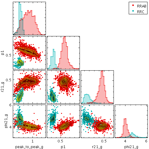
Example output from plot2corner.
The usage of plot2corner is
stilts <stilts-flags> plot2corner xpix=<int-value> ypix=<int-value>
insets=<top>,<left>,<bottom>,<right>
omode=swing|out|cgi|discard|auto
storage=simple|memory|disk|policy|cache|basic-cache|persistent|parallel
seq=<suffix>[,...] legend=true|false|null
legborder=true|false legopaque=true|false
legseq=<suffix>[,...]
legpos=<xfrac,yfrac> title=<value>
auxmap=<map-name>|<color>-<color>[-<color>...]
auxclip=<lo>,<hi> auxflip=true|false
auxquant=<number>
auxfunc=log|linear|histogram|...
auxmin=<number> auxmax=<number>
auxlabel=<text> auxcrowd=<factor>
auxwidth=<pixels>
auxvisible=true|false|null
forcebitmap=true|false compositor=0..1
animate=<table> afmt=<in-format>
astream=true|false acmd=<cmds>
parallel=<int-value> nvar=<int-value>
matrixformat=<value> cellgap=<int-value>
squares=true|false
xKscale=linear|log|asinh(<a>)|symlog(<t>,<s>)
xlog=true|false ylog=true|false
xKflip=true|false xKlabel=<text>
grid=true|false xcrowd=<number>
ycrowd=<number>
labelangle=horizontal|angled|adaptive
minor=true|false shadow=true|false
gridcolor=<rrggbb>|red|blue|...
gridtrans=0..1
labelcolor=<rrggbb>|red|blue|...
texttype=plain|antialias|latex
fontsize=<int-value>
fontstyle=standard|serif|mono
fontweight=plain|bold|italic|bold_italic
xKmin=<number> xKmax=<number>
xKsub=<lo>,<hi> navaxes=xy|x|y
xKanchor=true|false zoomfactor=<number>
leglabelN=<text>
layerN=<layer-type> <layerN-specific-params>
If you don't have the stilts script installed,
write "java -jar stilts.jar" instead of
"stilts" - see Section 3.
The available <stilts-flags> are listed
in Section 2.1.
For programmatic invocation,
the Task class for this
command is uk.ac.starlink.ttools.plot2.task.MatrixPlot2Task.
Parameter values are assigned on the command line as explained in Section 2.3. They are as follows:
acmd = <cmds> (ProcessingStep[])
animate,
before any other processing has taken place.
The value of this parameter is one or more of the filter
commands described in Section 6.1.
If more than one is given, they must be separated by
semicolon characters (";").
This parameter can be repeated multiple times on the same
command line to build up a list of processing steps.
The sequence of commands given in this way
defines the processing pipeline which is performed on the table.
Commands may alternatively be supplied in an external file,
by using the indirection character '@'.
Thus a value of "@filename"
causes the file filename to be read for a list
of filter commands to execute. The commands in the file
may be separated by newline characters and/or semicolons,
and lines which are blank or which start with a
'#' character are ignored.
A backslash character '\' at the end of a line
joins it with the following line.
afmt = <in-format> (String)
animate.
The known formats are listed in Section 5.1.1.
This flag can be used if you know what format your
table is in.
If it has the special value
(auto) (the default),
then an attempt will be
made to detect the format of the table automatically.
This cannot always be done correctly however, in which case
the program will exit with an error explaining which
formats were attempted.
This parameter is ignored for scheme-specified tables.
[Default: (auto)]
animate = <table> (StarTable)
The location of the animation control table. This may take one of the following forms:
-",
meaning standard input.
In this case the input format must be given explicitly
using the afmt
parameter.
Note that not all formats can be streamed in this way.:<scheme-name>:<scheme-args>.<" character at the start,
or a "|" character at the end
("<syscmd" or
"syscmd|").
This executes the given pipeline and reads from its
standard output.
This will probably only work on unix-like systems.astream = true|false (Boolean)
animate parameter
will be read as a stream.
It is necessary to give the
afmt parameter
in this case.
Depending on the required operations and processing mode,
this may cause the read to fail (sometimes it is necessary
to read the table more than once).
It is not normally necessary to set this flag;
in most cases the data will be streamed automatically
if that is the best thing to do.
However it can sometimes result in less resource usage when
processing large files in certain formats (such as VOTable).
This parameter is ignored for scheme-specified tables.
[Default: false]
auxclip = <lo>,<hi> (Subrange)
If the full range 0,1 is used,
the whole range of colours specified by the selected
shader will be used.
But if for instance a value of 0,0.5 is given,
only those colours at the left hand end of the ramp
will be seen.
If the null (default) value is chosen,
a default clip will be used.
This generally covers most or all of the range 0-1
but for colour maps which fade to white,
a small proportion of the lower end may be excluded,
to ensure that all the colours are visually distinguishable
from a white background.
This default is usually a good idea if the colour map
is being used with something like a scatter plot,
where markers are plotted against a white background.
However, for something like a density map when the whole
plotting area is tiled with colours from the map,
it may be better to supply the whole range
0,1 explicitly.
auxcrowd = <factor> (Double)
[Default: 1.0]
auxflip = true|false (Boolean)
[Default: false]
auxfunc = log|linear|histogram|... (Scaling)
The available options are:
log: Logarithmic scaling, positive values onlylinear: Linear scalinghistogram: Scaling follows data distribution, with linear axishistolog: Scaling follows data distribution, with logarithmic axis, positive values onlyasinh: Asinh scaling, wide dynamic range for both positive and negative valuessqrt: Square root scalingsquare: Square scalingacos: Inverse cosine Scalingcos: Cosine ScalingFor all these options,
the full range of valid data values is used,
and displayed on the colour bar
if applicable.
Note that logarithmic-based options
Log and
HistoLog
will ignore non-positive values.
The Linear,
Log,
Square and
Sqrt options
just apply the named function to the full data range.
The histogram options on the other hand use a scaling function
that corresponds to the actual distribution of the data, so that
there are about the same number of points (or pixels, or whatever
is being scaled) of each colour.
The histogram options are somewhat more expensive,
but can be a good choice if you are exploring data whose
distribution is unknown or not well-behaved over
its min-max range.
The Histogram and
HistoLog options both
assign the colours in the same way, but they display the colour
ramp with linear or logarithmic annotation respectively;
the HistoLog option also ignores
non-positive values.
[Default: linear]
auxlabel = <text> (String)
auxmap = <map-name>|<color>-<color>[-<color>...] (Shader)
A mixed bag of colour ramps are available
as listed in Section 8.7:
inferno,
magma,
plasma,
viridis,
cividis,
cubehelix,
sron,
rainbow,
rainbow2,
rainbow3,
pastel,
cosmic,
ember,
gothic,
rainforest,
voltage,
bubblegum,
gem,
chroma,
sunset,
neon,
tropical,
accent,
gnuplot,
gnuplot2,
specxby,
set1,
paired,
hotcold,
guppy,
iceburn,
redshift,
pride,
rdbu,
piyg,
brbg,
cyan-magenta,
red-blue,
brg,
heat,
cold,
light,
greyscale,
colour,
standard,
bugn,
bupu,
orrd,
pubu,
purd,
painbow,
huecl,
infinity,
hue,
intensity,
rgb_red,
rgb_green,
rgb_blue,
hsv_h,
hsv_s,
hsv_v,
yuv_y,
yuv_u,
yuv_v,
scale_hsv_s,
scale_hsv_v,
scale_yuv_y,
mask,
blacker,
whiter,
transparency.
Note:
many of these, including rainbow-like ones,
are frowned upon by the visualisation community.
You can also construct your own custom colour map
by giving a sequence of colour names separated by
minus sign ("-") characters.
In this case the ramp is a linear interpolation
between each pair of colours named,
using the same syntax as when specifying
a colour value.
So for instance
"yellow-hotpink-#0000ff"
would shade from yellow via hot pink to blue.
[Default: inferno]
auxmax = <number> (Double)
auxmin = <number> (Double)
auxquant = <number> (Double)
If left blank, the colour map is nominally continuous (though in practice it may be quantised to a medium-sized number like 256).
auxvisible = true|false|null (Boolean)
If not supplied (the default), the aux axis will be visible when aux shading is used in any of the plotted layers.
auxwidth = <pixels> (Integer)
[Default: 15]
cellgap = <int-value> (Integer)
[Default: 4]
compositor = 0..1 (Compositor)
Currently, this parameter takes a "boost" value in the range 0..1. If the value is zero, saturation semantics are used: RGB colours are added in proporition to their associated alpha value until the total alpha is saturated (reaches 1), after which additional pixels have no further effect. For larger boost values, the effect is similar, but any non-zero alpha in the output is boosted to the given minimum value. The effect of this is that even very slightly populated pixels can be visually distinguished from unpopulated ones which may not be the case for saturation composition.
[Default: 0.05]
fontsize = <int-value> (Integer)
[Default: 12]
fontstyle = standard|serif|mono (FontType)
The available options are:
standard
serif
mono
[Default: standard]
fontweight = plain|bold|italic|bold_italic (FontWeight)
The available options are:
plain
bold
italic
bold_italic
[Default: plain]
forcebitmap = true|false (Boolean)
shadingN=auto
or shadingN=density)
it will have no effect, since this kind of rendering
happens in any case.
When writing to vector graphics formats (PDF and PostScript), setting it true will force the data contents to be bitmapped. This may make the output less beautiful (round markers will no longer be perfectly round), but it may result in a much smaller file if there are very many data points.
When writing to bitmapped output formats (PNG, GIF, JPEG, ...), it fixes shapes to be the same as seen on the screen rather than be rendered at the mercy of the graphics system, which sometimes introduces small distortions.
[Default: false]
grid = true|false (Boolean)
[Default: false]
gridcolor = <rrggbb>|red|blue|... (Color)
The standard plotting colour names are
red, blue, green, grey, magenta, cyan, orange, pink, yellow, black, light_grey, white.
However, many other common colour names (too many to list here)
are also understood.
The list currently contains those colour names understood
by most web browsers,
from AliceBlue to YellowGreen,
listed e.g. in the
Extended color keywords section of
the CSS3 standard.
Alternatively, a six-digit hexadecimal number RRGGBB
may be supplied,
optionally prefixed by "#" or "0x",
giving red, green and blue intensities,
e.g. "ff00ff", "#ff00ff"
or "0xff00ff" for magenta.
[Default: grey]
gridtrans = 0..1 (Double)
[Default: 0.5]
insets = <top>,<left>,<bottom>,<right> (Padding)
The size and position of the actual plotting area
is determined by this parameter along with
xpix and
ypix.
The value of this parameter is 4 comma separated integers:
<top>,<left>,<bottom>,<right>.
Any or all of these values may be left blank,
in which case the corresponding margin will be calculated
automatically according to how much space is required.
labelangle = horizontal|angled|adaptive (OrientationPolicy)
Note that the adaptive
option is currently not perfect, and can sometimes lead to
suboptimal border placement.
The available options are:
horizontal: axis labels are horizontalangled: axis labels are angledadaptive: axis labels are horizontal if possible, but angled if necessary to fit more in[Default: angled]
labelcolor = <rrggbb>|red|blue|... (Color)
The standard plotting colour names are
red, blue, green, grey, magenta, cyan, orange, pink, yellow, black, light_grey, white.
However, many other common colour names (too many to list here)
are also understood.
The list currently contains those colour names understood
by most web browsers,
from AliceBlue to YellowGreen,
listed e.g. in the
Extended color keywords section of
the CSS3 standard.
Alternatively, a six-digit hexadecimal number RRGGBB
may be supplied,
optionally prefixed by "#" or "0x",
giving red, green and blue intensities,
e.g. "ff00ff", "#ff00ff"
or "0xff00ff" for magenta.
[Default: black]
layerN = <layer-type> <layerN-specific-params> (LayerType)
layer<N>
where the suffix "<N>"
is a label identifying the layer
and is appended to all the parameter names
which configure that layer.
Suffixes may be any string, including the empty string.
This parameter may take one of the following values, described in more detail in Section 8.3:
Each of these layer types comes with a list of type-specific parameters to define the details of that layer, including some or all of the following groups:
inN,
icmdN)xN,
yN)shadingN,
colorN)Every parameter notionally carries the same suffix
N.
However, if the suffix is not present,
the application will try looking for a parameter with the
same name with no suffix instead.
In this way, if several layers have the same value for a given
parameter (for instance input table),
you can supply it using one unsuffixed parameter
to save having to supply several parameters with the same
value but different suffixes.
legborder = true|false (Boolean)
[Default: true]
legend = true|false|null (Boolean)
leglabelN = <text> (String)
If no value is supplied (the default), the suffix itself is used as the label.
legopaque = true|false (Boolean)
[Default: true]
legpos = <xfrac,yfrac> (double[])
0.5,0.5" will put the legend
right in the middle of the plot.
If no value is supplied, the legend will appear outside
the plot boundary.
legseq = <suffix>[,...] (String[])
leglabelN
parameter).
If multiple layers have the same label,
they will contribute to the same entry in the legend,
with style icons plotted over each other.
The value of this parameter is a comma-separated sequence
of layer suffixes,
which determines the order in which the legend entries appear.
Layers with suffixes missing from this list
do not show up in the legend at all.
If no value is supplied (the default),
the sequence is the same as the layer plotting sequence
(see seq).
matrixformat = <value> (MatrixFormat)
The available options are:
lower: only the lower diagonal part of the matrix is populated, as well as the diagonal if diagonal elements are presentupper: only the upper diagonal part of the matrix is populated, as well as the diagonal if diagonal elements are presentfull: all cells of the matrix are populated where present[Default: lower]
minor = true|false (Boolean)
[Default: true]
navaxes = xy|x|y (boolean[])
xy, which means that
the various mouse gestures will provide panning and zooming
in both X and Y directions.
However, if it is set to (for instance) x
then the mouse will only allow panning and
zooming in the horizontal direction,
with the vertical extent fixed.
[Default: xy]
nvar = <int-value> (Integer)
[Default: 3]
omode = swing|out|cgi|discard|auto (PaintMode)
swing:
Plot will be displayed in a window on the screen.
This plot is "live"; it can be resized and (except for old-style plots)
navigated around with mouse actions in the same way as plots in TOPCAT.out:
Plot will be written to a file given by out using the graphics format given by ofmt.cgi:
Plot will be written in a way suitable for CGI use direct from a web server.
The output is in the graphics format given by ofmt,
preceded by a suitable "Content-type" declaration.discard:
Plot is drawn, but discarded. There is no output.auto:
Behaves as swing or out mode depending on presence of out parameter[Default: auto]
parallel = <int-value> (Integer)
animate
parameter is supplied.
The default value is the number of processors apparently
available to the JVM.
[Default: 20]
seq = <suffix>[,...] (String[])
When specifying a plot, multiple layers may be specified,
each introduced by a parameter
layer<N>,
where <N> is a different (arbitrary)
suffix labelling the layer,
and is appended to all the parameters
specific to defining that layer.
By default the layers are drawn on the plot in the order
in which the layer* parameters
appear on the command line.
However if this parameter is specified, each comma-separated
element is interpreted as a layer suffix,
giving the ordered list of layers to plot.
Every element of the list must be a suffix with a corresponding
layer parameter,
but missing or repeated elements are allowed.
shadow = true|false (Boolean)
[Default: true]
squares = true|false (Boolean)
[Default: false]
storage = simple|memory|disk|policy|cache|basic-cache|persistent|parallel (DataStoreFactory)
The options are:
simple:
no caching, data read directly from input table
memory:
cached to memory; OutOfMemoryError possible
for very large plots
disk:
cached to disk
policy:
cached using application-wide default storage policy,
which is usually adaptive (memory/disk hybrid)
persistent:
cached to persistent files on disk,
in the system temporary directory
(defined by system property java.io.tmpdir).
If this is used, plot data will be stored on disk in a way
that means they can be re-used between STILTS invocations,
so data preparation can be avoided on subsequent runs.
Note however it can leave potentially large files
in your temporary directory.
cache:
synonym for memory (backward compatibility)
basic-cache:
dumber version of memory
(no optimisation for constant-valued columns)
parallel:
experimental version of memory-based cache that reads
into the cache in parallel for large files.
This will make the plot faster to prepare,
but interaction is a bit slower and sequence-dependent
attributes of the plot may not come out right.
This experimental option may be withdrawn or modified
in future releases.
The default value is
memory
if a live plot is being generated
(omode=swing),
since in that case the plot needs to be redrawn every time
the user performs plot navigation actions or resizes the window,
or if animations are being produced.
Otherwise (e.g. output to a graphics file) the default is
simple.
[Default: simple]
texttype = plain|antialias|latex (TextSyntax)
Plain and
Antialias
both take the text at face value,
but Antialias
smooths the characters.
LaTeX
interprets the text as LaTeX source code
and typesets it accordingly.
When not using LaTeX, antialiased text usually looks nicer, but can be perceptibly slower to plot. At time of writing, on MacOS antialiased text seems to be required to stop the writing coming out upside-down for non-horizontal text (MacOS java bug).
[Default: plain]
title = <value> (String)
xKanchor = true|false (Boolean)
The xK axis refers to any axes in the matrix
on which input coordinate #K is plotted.
Hence
x2anchor
affects the axes on which the x2 coordinates
are plotted.
[Default: false]
xKflip = true|false (Boolean)
The xK axis refers to any axes in the matrix
on which input coordinate #K is plotted.
Hence
x2flip
affects the axes on which the x2 coordinates
are plotted.
[Default: false]
xKlabel = <text> (String)
The xK axis refers to any axes in the matrix
on which input coordinate #K is plotted.
Hence
x2label
affects the axes on which the x2 coordinates
are plotted.
[Default: xK]
xKmax = <number> (Double)
The xK axis refers to any axes in the matrix
on which input coordinate #K is plotted.
Hence
x2max
affects the axes on which the x2 coordinates
are plotted.
xKmin = <number> (Double)
The xK axis refers to any axes in the matrix
on which input coordinate #K is plotted.
Hence
x2min
affects the axes on which the x2 coordinates
are plotted.
xKscale = linear|log|asinh(<a>)|symlog(<t>,<s>) (Scale)
linear: Linear scalelog: Logarithmic scaleasinh: Scaling based on inverse hyperbolic sin function.
This is approximately linear near the origin,
and approximately logarithmic far from it.
It has one parameter, the "linear width" a,
which controls the extent of the linear-like region,
and must be strictly positive.
The function is x->asinh(x/a).symlog: Symmetric logarithmic scale.
This is linear near the origin, and positive/negative
logarithmic for larger values.
It has two parameters,
t (a.k.a. linthresh) and
s (a.k.a. linscale).
Both parameters must be strictly positive.
The linear region is in the range
-t<x<+t,
and the graphical extent of the region from the origin
to t is the same as
s decades in the logarithmic region.For those options which have parameters,
the values are specified after the name in brackets,
e.g. "symlog(10,0.5)".
If the parameters are missing (e.g. "symlog")
some default values are used.
The linear and log options
should be self-explanatory.
symlog and asinh allow plots over
a wide dynamic range like log,
but unlike log they can accommodate
negative as well as positive values.
In both cases scaling near the origin is more or less linear
(like x),
and scaling far from the origin is more or less logarithmic,
(like (log(x) or -log(-x)).
The symlog option simply switches between the
two regimes at a given threshold,
while asinh transitions smoothly.
These options were copied from the equivalent functionality in
matplotlib.
The xK axis refers to any axes in the matrix
on which input coordinate #K is plotted.
Hence
x2scale
affects the axes on which the x2 coordinates
are plotted.
[Default: linear]
xKsub = <lo>,<hi> (Subrange)
The default value "0,1" therefore has
no effect.
The range could be restricted to its lower half
with the value 0,0.5.
The xK axis refers to any axes in the matrix
on which input coordinate #K is plotted.
Hence
x2sub
affects the axes on which the x2 coordinates
are plotted.
[Default: 0,1]
xcrowd = <number> (Double)
[Default: 1]
xlog = true|false (Boolean)
Note this option is deprecated in favour of
the xscale option,
which offers more flexible axis scaling options.
[Default: false]
xpix = <int-value> (Integer)
insets.
[Default: 500]
ycrowd = <number> (Double)
[Default: 1]
ylog = true|false (Boolean)
Note this option is deprecated in favour of
the yscale option,
which offers more flexible axis scaling options.
[Default: false]
ypix = <int-value> (Integer)
insets.
[Default: 400]
zoomfactor = <number> (Double)
[Default: 1.2]
Here are some examples of using plot2corner:
stilts plot2corner in=:attractor:100000,rampe
nvar=3 x1=x x2=y x3=z
layer_m=mark
stilts plot2corner in=:attractor:100000,rampe
nvar=3 x1=x x2=y x3=z
matrixformat=full
layer_m=mark layer_h=histogram
matrixformat=full parameter
means that the full grid (with redundant plots also for
Y vs. X, Z vs. X, and Z vs. Y) are plotted above the diagonal.
stilts plot2corner in=rrlyrae.fits
icmd_A='select best_classification==\"RRAB\"'
icmd_C='select best_classification==\"RRC\"'
color_A=red color_C=cyan
nvar=4 x1=peak_to_peak_g x2=p1 x3=r21_g x4=phi21_g x4min=3
layer_A_m=mark layer_C_m=mark
layer_A_k=kde layer_C_k=kde smooth_A_k=-50 smooth_C_k=-50
layer_f=contour color_f=light_grey smooth_f=10 nlevel_f=6
leglabel_A=RRAB leglabel_C=RRC legseq=_A_m,_C_m legpos=1,1
x4min parameter.
As well as the mark and kde layers,
an additional contour layer (of the whole input table)
is overplotted on the scatter plot grid elements.
plot2time: Draws a time plot
plot2time draws plots where the horizontal axis represents time.
The time axis can be labelled in various different ways including
MJD, decimal year and ISO-8601 form.
Positional coordinates are specified as t, y pairs,
with an optional ttype specifier to indicate how the
input value is to be interpreted,
e.g.:
plot2time in1=series.fits layer1=line t1=EPOCH ttype1=MJD y1=ENERGY
Time values can be represented in various ways in input data,
for instance as Julian Day, Modified Julian Date, decimal years
since 0AD, Unix seconds, ISO-8601, or variants of some of the
above with additional offsets.
In some cases the input format contains enough metadata to
determine how the values should be mapped to a common timescale
(so for instance they can be plotted as MJD or Year/Month/Day),
and in other cases they do not.
For example CDF files and VOTable 1.4 files with TIMESYS
markup contain sufficient metadata, and text inputs using the
ISO-8601 format can usually be identified and understood,
but there's no way to tell automatically whether a numeric column
in a CSV file represents MJD, seconds since a known epoch,
decimal years, or anything else.
For this reason the ttypeN parameter is provided
for all the layer types with a tN coordinate,
as follows:
ttypeN = DecYear|MJD|JD|Unix|Iso8601 (TimeMapper)
tN is supplied.
Options are:
DecYear: Years since 0 ADMJD: Modified Julian DateJD: Julian DayUnix: Seconds since midnight 1 Jan 1970Iso8601: ISO 8601 stringtN value.
This command,
unlike the other plot2* commands at time of writing,
can be used to draw multi-zone plots.
These are plots with different panels stacked vertically so that
different datasets can share the same horizontal (time) axis, but have
separate vertical axes, colour maps, legends etc.
The horizontal axes are always synchronized between zones.
This is currently controlled with the zoneN parameter.
For any layer with a layer suffix N, you can specify
a zone identifier as an arbitrary string, Z,
by supplying the parameter zoneN=Z.
Layers with the same value of
zoneN are plotted in the same zone, and layers with
different values are plotted in different zones.
If no zoneN is given, the layer is assigned to
a single (unnamed) zone, so with no zone parameters specified
all plots appear in a single zone.
Parameters specific to a given zone can then be suffixed with the
same Z zone identifier.
The examples section illustrates
what this looks like in practice.
Note: The multi-zone feature is experimental. As currently implemented it lacks some features. The interface may be changed in a future version.
Content is added to the plot by specifying
one or more plot layers using the
layerN parameter.
The N part is a suffix applied to
all the parameters affecting a given layer;
any suffix (including the empty string) may be used.
Available layers for this plot type are:
line,
linearfit,
mark,
fill,
quantile,
grid,
histogram,
kde,
knn,
densogram,
gaussian,
yerror,
spectrogram,
label,
function.
The usage of plot2time is
stilts <stilts-flags> plot2time xpix=<int-value> ypix=<int-value>
insets=<top>,<left>,<bottom>,<right>
omode=swing|out|cgi|discard|auto
storage=simple|memory|disk|policy|cache|basic-cache|persistent|parallel
seq=<suffix>[,...] legend=true|false|null
legborder=true|false legopaque=true|false
legseq=<suffix>[,...] legpos=<xfrac,yfrac>
title=<value>
auxmap=<map-name>|<color>-<color>[-<color>...]
auxclip=<lo>,<hi> auxflip=true|false
auxquant=<number>
auxfunc=log|linear|histogram|...
auxmin=<number> auxmax=<number>
auxlabel=<text> auxcrowd=<factor>
auxwidth=<pixels>
auxvisible=true|false|null
forcebitmap=true|false compositor=0..1
animate=<table> afmt=<in-format>
astream=true|false acmd=<cmds>
parallel=<int-value> cellgap=<int-value>
yscale=linear|log|asinh(<a>)|symlog(<t>,<s>)
ylog=true|false yflip=true|false
tlabel=<text> ylabel=<text>
t2func=<time-expr> y2func=<function-of-y>
t2label=<text> y2label=<text>
grid=true|false tcrowd=<number>
ycrowd=<number>
labelangle=horizontal|angled|adaptive
tformat=iso-8601|year|mjd|unix
minor=true|false shadow=true|false
gridcolor=<rrggbb>|red|blue|...
gridtrans=0..1
texttype=plain|antialias|latex
fontsize=<int-value>
fontstyle=standard|serif|mono
fontweight=plain|bold|italic|bold_italic
tmin=<year-or-iso8601>
tmax=<year-or-iso8601> tsub=<lo>,<hi>
ymin=<number> ymax=<number> ysub=<lo>,<hi>
navaxes=t|y|ty zoomfactor=<number>
leglabelN=<text>
layerN=<layer-type> <layerN-specific-params>
zoneN=<text>
If you don't have the stilts script installed,
write "java -jar stilts.jar" instead of
"stilts" - see Section 3.
The available <stilts-flags> are listed
in Section 2.1.
For programmatic invocation,
the Task class for this
command is uk.ac.starlink.ttools.plot2.task.TimePlot2Task.
Parameter values are assigned on the command line as explained in Section 2.3. They are as follows:
acmd = <cmds> (ProcessingStep[])
animate,
before any other processing has taken place.
The value of this parameter is one or more of the filter
commands described in Section 6.1.
If more than one is given, they must be separated by
semicolon characters (";").
This parameter can be repeated multiple times on the same
command line to build up a list of processing steps.
The sequence of commands given in this way
defines the processing pipeline which is performed on the table.
Commands may alternatively be supplied in an external file,
by using the indirection character '@'.
Thus a value of "@filename"
causes the file filename to be read for a list
of filter commands to execute. The commands in the file
may be separated by newline characters and/or semicolons,
and lines which are blank or which start with a
'#' character are ignored.
A backslash character '\' at the end of a line
joins it with the following line.
afmt = <in-format> (String)
animate.
The known formats are listed in Section 5.1.1.
This flag can be used if you know what format your
table is in.
If it has the special value
(auto) (the default),
then an attempt will be
made to detect the format of the table automatically.
This cannot always be done correctly however, in which case
the program will exit with an error explaining which
formats were attempted.
This parameter is ignored for scheme-specified tables.
[Default: (auto)]
animate = <table> (StarTable)
The location of the animation control table. This may take one of the following forms:
-",
meaning standard input.
In this case the input format must be given explicitly
using the afmt
parameter.
Note that not all formats can be streamed in this way.:<scheme-name>:<scheme-args>.<" character at the start,
or a "|" character at the end
("<syscmd" or
"syscmd|").
This executes the given pipeline and reads from its
standard output.
This will probably only work on unix-like systems.astream = true|false (Boolean)
animate parameter
will be read as a stream.
It is necessary to give the
afmt parameter
in this case.
Depending on the required operations and processing mode,
this may cause the read to fail (sometimes it is necessary
to read the table more than once).
It is not normally necessary to set this flag;
in most cases the data will be streamed automatically
if that is the best thing to do.
However it can sometimes result in less resource usage when
processing large files in certain formats (such as VOTable).
This parameter is ignored for scheme-specified tables.
[Default: false]
auxclip = <lo>,<hi> (Subrange)
If the full range 0,1 is used,
the whole range of colours specified by the selected
shader will be used.
But if for instance a value of 0,0.5 is given,
only those colours at the left hand end of the ramp
will be seen.
If the null (default) value is chosen,
a default clip will be used.
This generally covers most or all of the range 0-1
but for colour maps which fade to white,
a small proportion of the lower end may be excluded,
to ensure that all the colours are visually distinguishable
from a white background.
This default is usually a good idea if the colour map
is being used with something like a scatter plot,
where markers are plotted against a white background.
However, for something like a density map when the whole
plotting area is tiled with colours from the map,
it may be better to supply the whole range
0,1 explicitly.
If a zone suffix is appended to the parameter name,
only that zone is affected,
e.g. auxclipZ affects only zone Z.
auxcrowd = <factor> (Double)
If a zone suffix is appended to the parameter name, only that zone is affected,
e.g. auxcrowdZ affects only zone Z.
[Default: 1.0]
auxflip = true|false (Boolean)
If a zone suffix is appended to the parameter name,
only that zone is affected,
e.g. auxflipZ affects only zone Z.
[Default: false]
auxfunc = log|linear|histogram|... (Scaling)
The available options are:
log: Logarithmic scaling, positive values onlylinear: Linear scalinghistogram: Scaling follows data distribution, with linear axishistolog: Scaling follows data distribution, with logarithmic axis, positive values onlyasinh: Asinh scaling, wide dynamic range for both positive and negative valuessqrt: Square root scalingsquare: Square scalingacos: Inverse cosine Scalingcos: Cosine ScalingFor all these options,
the full range of valid data values is used,
and displayed on the colour bar
if applicable.
Note that logarithmic-based options
Log and
HistoLog
will ignore non-positive values.
The Linear,
Log,
Square and
Sqrt options
just apply the named function to the full data range.
The histogram options on the other hand use a scaling function
that corresponds to the actual distribution of the data, so that
there are about the same number of points (or pixels, or whatever
is being scaled) of each colour.
The histogram options are somewhat more expensive,
but can be a good choice if you are exploring data whose
distribution is unknown or not well-behaved over
its min-max range.
The Histogram and
HistoLog options both
assign the colours in the same way, but they display the colour
ramp with linear or logarithmic annotation respectively;
the HistoLog option also ignores
non-positive values.
If a zone suffix is appended to the parameter name,
only that zone is affected,
e.g. auxfuncZ affects only zone Z.
[Default: linear]
auxlabel = <text> (String)
If a zone suffix is appended to the parameter name, only that zone is affected,
e.g. auxlabelZ affects only zone Z.
auxmap = <map-name>|<color>-<color>[-<color>...] (Shader)
A mixed bag of colour ramps are available
as listed in Section 8.7:
inferno,
magma,
plasma,
viridis,
cividis,
cubehelix,
sron,
rainbow,
rainbow2,
rainbow3,
pastel,
cosmic,
ember,
gothic,
rainforest,
voltage,
bubblegum,
gem,
chroma,
sunset,
neon,
tropical,
accent,
gnuplot,
gnuplot2,
specxby,
set1,
paired,
hotcold,
guppy,
iceburn,
redshift,
pride,
rdbu,
piyg,
brbg,
cyan-magenta,
red-blue,
brg,
heat,
cold,
light,
greyscale,
colour,
standard,
bugn,
bupu,
orrd,
pubu,
purd,
painbow,
huecl,
infinity,
hue,
intensity,
rgb_red,
rgb_green,
rgb_blue,
hsv_h,
hsv_s,
hsv_v,
yuv_y,
yuv_u,
yuv_v,
scale_hsv_s,
scale_hsv_v,
scale_yuv_y,
mask,
blacker,
whiter,
transparency.
Note:
many of these, including rainbow-like ones,
are frowned upon by the visualisation community.
You can also construct your own custom colour map
by giving a sequence of colour names separated by
minus sign ("-") characters.
In this case the ramp is a linear interpolation
between each pair of colours named,
using the same syntax as when specifying
a colour value.
So for instance
"yellow-hotpink-#0000ff"
would shade from yellow via hot pink to blue.
If a zone suffix is appended to the parameter name,
only that zone is affected,
e.g. auxmapZ affects only zone Z.
[Default: inferno]
auxmax = <number> (Double)
If a zone suffix is appended to the parameter name,
only that zone is affected,
e.g. auxmaxZ affects only zone Z.
auxmin = <number> (Double)
If a zone suffix is appended to the parameter name,
only that zone is affected,
e.g. auxminZ affects only zone Z.
auxquant = <number> (Double)
If left blank, the colour map is nominally continuous (though in practice it may be quantised to a medium-sized number like 256).
If a zone suffix is appended to the parameter name,
only that zone is affected,
e.g. auxquantZ affects only zone Z.
auxvisible = true|false|null (Boolean)
If not supplied (the default), the aux axis will be visible when aux shading is used in any of the plotted layers.
If a zone suffix is appended to the parameter name, only that zone is affected,
e.g. auxvisibleZ affects only zone Z.
auxwidth = <pixels> (Integer)
If a zone suffix is appended to the parameter name, only that zone is affected,
e.g. auxwidthZ affects only zone Z.
[Default: 15]
cellgap = <int-value> (Integer)
[Default: 4]
compositor = 0..1 (Compositor)
Currently, this parameter takes a "boost" value in the range 0..1. If the value is zero, saturation semantics are used: RGB colours are added in proporition to their associated alpha value until the total alpha is saturated (reaches 1), after which additional pixels have no further effect. For larger boost values, the effect is similar, but any non-zero alpha in the output is boosted to the given minimum value. The effect of this is that even very slightly populated pixels can be visually distinguished from unpopulated ones which may not be the case for saturation composition.
[Default: 0.05]
fontsize = <int-value> (Integer)
If a zone suffix is appended to the parameter name,
only that zone is affected,
e.g. fontsizeZ affects only zone Z.
[Default: 12]
fontstyle = standard|serif|mono (FontType)
The available options are:
standard
serif
mono
If a zone suffix is appended to the parameter name,
only that zone is affected,
e.g. fontstyleZ affects only zone Z.
[Default: standard]
fontweight = plain|bold|italic|bold_italic (FontWeight)
The available options are:
plain
bold
italic
bold_italic
If a zone suffix is appended to the parameter name,
only that zone is affected,
e.g. fontweightZ affects only zone Z.
[Default: plain]
forcebitmap = true|false (Boolean)
shadingN=auto
or shadingN=density)
it will have no effect, since this kind of rendering
happens in any case.
When writing to vector graphics formats (PDF and PostScript), setting it true will force the data contents to be bitmapped. This may make the output less beautiful (round markers will no longer be perfectly round), but it may result in a much smaller file if there are very many data points.
When writing to bitmapped output formats (PNG, GIF, JPEG, ...), it fixes shapes to be the same as seen on the screen rather than be rendered at the mercy of the graphics system, which sometimes introduces small distortions.
[Default: false]
grid = true|false (Boolean)
If a zone suffix is appended to the parameter name,
only that zone is affected,
e.g. gridZ affects only zone Z.
[Default: false]
gridcolor = <rrggbb>|red|blue|... (Color)
The standard plotting colour names are
red, blue, green, grey, magenta, cyan, orange, pink, yellow, black, light_grey, white.
However, many other common colour names (too many to list here)
are also understood.
The list currently contains those colour names understood
by most web browsers,
from AliceBlue to YellowGreen,
listed e.g. in the
Extended color keywords section of
the CSS3 standard.
Alternatively, a six-digit hexadecimal number RRGGBB
may be supplied,
optionally prefixed by "#" or "0x",
giving red, green and blue intensities,
e.g. "ff00ff", "#ff00ff"
or "0xff00ff" for magenta.
If a zone suffix is appended to the parameter name,
only that zone is affected,
e.g. gridcolorZ affects only zone Z.
[Default: grey]
gridtrans = 0..1 (Double)
If a zone suffix is appended to the parameter name,
only that zone is affected,
e.g. gridtransZ affects only zone Z.
[Default: 0.5]
insets = <top>,<left>,<bottom>,<right> (Padding)
The size and position of the actual plotting area
is determined by this parameter along with
xpix and
ypix.
The value of this parameter is 4 comma separated integers:
<top>,<left>,<bottom>,<right>.
Any or all of these values may be left blank,
in which case the corresponding margin will be calculated
automatically according to how much space is required.
labelangle = horizontal|angled|adaptive (OrientationPolicy)
Note that the adaptive
option is currently not perfect, and can sometimes lead to
suboptimal border placement.
The available options are:
horizontal: axis labels are horizontalangled: axis labels are angledadaptive: axis labels are horizontal if possible, but angled if necessary to fit more inIf a zone suffix is appended to the parameter name,
only that zone is affected,
e.g. labelangleZ affects only zone Z.
[Default: horizontal]
layerN = <layer-type> <layerN-specific-params> (LayerType)
layer<N>
where the suffix "<N>"
is a label identifying the layer
and is appended to all the parameter names
which configure that layer.
Suffixes may be any string, including the empty string.
This parameter may take one of the following values, described in more detail in Section 8.3:
line
linearfit
mark
fill
quantile
grid
histogram
kde
knn
densogram
gaussian
yerror
spectrogram
label
function
Each of these layer types comes with a list of type-specific parameters to define the details of that layer, including some or all of the following groups:
inN,
icmdN)xN,
yN)shadingN,
colorN)Every parameter notionally carries the same suffix
N.
However, if the suffix is not present,
the application will try looking for a parameter with the
same name with no suffix instead.
In this way, if several layers have the same value for a given
parameter (for instance input table),
you can supply it using one unsuffixed parameter
to save having to supply several parameters with the same
value but different suffixes.
legborder = true|false (Boolean)
[Default: true]
legend = true|false|null (Boolean)
leglabelN = <text> (String)
If no value is supplied (the default), the suffix itself is used as the label.
legopaque = true|false (Boolean)
[Default: true]
legpos = <xfrac,yfrac> (double[])
0.5,0.5" will put the legend
right in the middle of the plot.
If no value is supplied, the legend will appear outside
the plot boundary.
If a zone suffix is appended to the parameter name, only that zone is affected,
e.g. legposZ affects only zone Z.
legseq = <suffix>[,...] (String[])
leglabelN
parameter).
If multiple layers have the same label,
they will contribute to the same entry in the legend,
with style icons plotted over each other.
The value of this parameter is a comma-separated sequence
of layer suffixes,
which determines the order in which the legend entries appear.
Layers with suffixes missing from this list
do not show up in the legend at all.
If no value is supplied (the default),
the sequence is the same as the layer plotting sequence
(see seq).
minor = true|false (Boolean)
If a zone suffix is appended to the parameter name,
only that zone is affected,
e.g. minorZ affects only zone Z.
[Default: true]
navaxes = t|y|ty (boolean[])
t
which means that the various mouse gestures
will provide panning and zooming in the Time direction only.
However, if it is set to ty
mouse actions will affect both the horizontal and vertical
axes.
[Default: t]
omode = swing|out|cgi|discard|auto (PaintMode)
swing:
Plot will be displayed in a window on the screen.
This plot is "live"; it can be resized and (except for old-style plots)
navigated around with mouse actions in the same way as plots in TOPCAT.out:
Plot will be written to a file given by out using the graphics format given by ofmt.cgi:
Plot will be written in a way suitable for CGI use direct from a web server.
The output is in the graphics format given by ofmt,
preceded by a suitable "Content-type" declaration.discard:
Plot is drawn, but discarded. There is no output.auto:
Behaves as swing or out mode depending on presence of out parameter[Default: auto]
parallel = <int-value> (Integer)
animate
parameter is supplied.
The default value is the number of processors apparently
available to the JVM.
[Default: 20]
seq = <suffix>[,...] (String[])
When specifying a plot, multiple layers may be specified,
each introduced by a parameter
layer<N>,
where <N> is a different (arbitrary)
suffix labelling the layer,
and is appended to all the parameters
specific to defining that layer.
By default the layers are drawn on the plot in the order
in which the layer* parameters
appear on the command line.
However if this parameter is specified, each comma-separated
element is interpreted as a layer suffix,
giving the ordered list of layers to plot.
Every element of the list must be a suffix with a corresponding
layer parameter,
but missing or repeated elements are allowed.
shadow = true|false (Boolean)
If a zone suffix is appended to the parameter name,
only that zone is affected,
e.g. shadowZ affects only zone Z.
[Default: true]
storage = simple|memory|disk|policy|cache|basic-cache|persistent|parallel (DataStoreFactory)
The options are:
simple:
no caching, data read directly from input table
memory:
cached to memory; OutOfMemoryError possible
for very large plots
disk:
cached to disk
policy:
cached using application-wide default storage policy,
which is usually adaptive (memory/disk hybrid)
persistent:
cached to persistent files on disk,
in the system temporary directory
(defined by system property java.io.tmpdir).
If this is used, plot data will be stored on disk in a way
that means they can be re-used between STILTS invocations,
so data preparation can be avoided on subsequent runs.
Note however it can leave potentially large files
in your temporary directory.
cache:
synonym for memory (backward compatibility)
basic-cache:
dumber version of memory
(no optimisation for constant-valued columns)
parallel:
experimental version of memory-based cache that reads
into the cache in parallel for large files.
This will make the plot faster to prepare,
but interaction is a bit slower and sequence-dependent
attributes of the plot may not come out right.
This experimental option may be withdrawn or modified
in future releases.
The default value is
memory
if a live plot is being generated
(omode=swing),
since in that case the plot needs to be redrawn every time
the user performs plot navigation actions or resizes the window,
or if animations are being produced.
Otherwise (e.g. output to a graphics file) the default is
simple.
[Default: simple]
t2func = <time-expr> (TimeJELFunction)
The value of this parameter is an algebraic expression giving the numeric value to be displayed on the secondary axis corresponding to a given time value on the primary axis. The expression may be given in terms of one of the following variables:
mjd: Modified Julian Datejd: Julian DaydecYear: decimal year CEunixSec: seconds since 1970-01-01T00:00:00In most cases, the value of this parameter will simply be
one of those variable names, for instance,
"mjd" to annotate the secondary axis
in Modified Julian Date.
However you can apply operations to these values in the usual way
if required, for instance to provide a differently offset
date scale.
The function supplied should be monotonic and reasonably well-behaved, otherwise the secondary axis annotation may not work well. Tick marks will always be applied on a linear scale. Currently there is no way to annotate the secondary axis with ISO-8601 dates or other non-numeric labels.
If a zone suffix is appended to the parameter name,
only that zone is affected,
e.g. t2funcZ affects only zone Z.
t2label = <text> (String)
If a zone suffix is appended to the parameter name,
only that zone is affected,
e.g. t2labelZ affects only zone Z.
tcrowd = <number> (Double)
If a zone suffix is appended to the parameter name,
only that zone is affected,
e.g. tcrowdZ affects only zone Z.
[Default: 1]
texttype = plain|antialias|latex (TextSyntax)
Plain and
Antialias
both take the text at face value,
but Antialias
smooths the characters.
LaTeX
interprets the text as LaTeX source code
and typesets it accordingly.
When not using LaTeX, antialiased text usually looks nicer, but can be perceptibly slower to plot. At time of writing, on MacOS antialiased text seems to be required to stop the writing coming out upside-down for non-horizontal text (MacOS java bug).
If a zone suffix is appended to the parameter name,
only that zone is affected,
e.g. texttypeZ affects only zone Z.
[Default: plain]
tformat = iso-8601|year|mjd|unix (TimeFormat)
The available options are:
iso-8601: ISO 8601 date, of the form yyyy-mm-ddThh:mm:ss.s (e.g. "2012-03-13T04")year: Decimal year (e.g. "2012.197")mjd: Modified Julian Date (e.g. "55999.2")unix: Seconds since midnight of 1 Jan 1970 (e.g. "1331613420")If a zone suffix is appended to the parameter name,
only that zone is affected,
e.g. tformatZ affects only zone Z.
[Default: iso-8601]
title = <value> (String)
If a zone suffix is appended to the parameter name, only that zone is affected,
e.g. titleZ affects only zone Z.
tlabel = <text> (String)
If a zone suffix is appended to the parameter name,
only that zone is affected,
e.g. tlabelZ affects only zone Z.
tmax = <year-or-iso8601> (Double)
The value may be set with a string that can be interpreted as
a decimal year
(e.g. "2007.521")
or an ISO-8601 string
(e.g. "2007-07-10T03:57:36",
"2007-07-10T03"
or "2007-07-10").
Note however that the numeric value of this configuration item
if accessed programmatically is seconds since 1 Jan 1970.
If a zone suffix is appended to the parameter name,
only that zone is affected,
e.g. tmaxZ affects only zone Z.
tmin = <year-or-iso8601> (Double)
The value may be set with a string that can be interpreted as
a decimal year
(e.g. "2007.521")
or an ISO-8601 string
(e.g. "2007-07-10T03:57:36",
"2007-07-10T03"
or "2007-07-10").
Note however that the numeric value of this configuration item
if accessed programmatically is seconds since 1 Jan 1970.
If a zone suffix is appended to the parameter name,
only that zone is affected,
e.g. tminZ affects only zone Z.
tsub = <lo>,<hi> (Subrange)
The default value "0,1" therefore has
no effect.
The range could be restricted to its lower half
with the value 0,0.5.
If a zone suffix is appended to the parameter name,
only that zone is affected,
e.g. tsubZ affects only zone Z.
[Default: 0,1]
xpix = <int-value> (Integer)
insets.
[Default: 500]
y2func = <function-of-y> (JELFunction)
The value of this parameter is an
algebraic expression in terms of the variable
y giving the value
on the secondary Y axis
corresponding to a given value
on the primary Y axis.
For instance, if the primary Y axis
represents flux in Jansky,
then supplying the expression
"2.5*(23-log10(y))-48.6"
(or "janskyToAb(y)")
would annotate the secondary Y axis
as AB magnitudes.
The function supplied should be monotonic and reasonably well-behaved, otherwise the secondary axis annotation may not work well. The application will attempt to make a sensible decision about whether to use linear or logarithmic tick marks.
If a zone suffix is appended to the parameter name,
only that zone is affected,
e.g. y2funcZ affects only zone Z.
y2label = <text> (String)
If a zone suffix is appended to the parameter name,
only that zone is affected,
e.g. y2labelZ affects only zone Z.
ycrowd = <number> (Double)
If a zone suffix is appended to the parameter name,
only that zone is affected,
e.g. ycrowdZ affects only zone Z.
[Default: 1]
yflip = true|false (Boolean)
If a zone suffix is appended to the parameter name,
only that zone is affected,
e.g. yflipZ affects only zone Z.
[Default: false]
ylabel = <text> (String)
If a zone suffix is appended to the parameter name,
only that zone is affected,
e.g. ylabelZ affects only zone Z.
[Default: Y]
ylog = true|false (Boolean)
Note this option is deprecated in favour of
the yscale option,
which offers more flexible axis scaling options.
If a zone suffix is appended to the parameter name,
only that zone is affected,
e.g. ylogZ affects only zone Z.
[Default: false]
ymax = <number> (Double)
If a zone suffix is appended to the parameter name,
only that zone is affected,
e.g. ymaxZ affects only zone Z.
ymin = <number> (Double)
If a zone suffix is appended to the parameter name,
only that zone is affected,
e.g. yminZ affects only zone Z.
ypix = <int-value> (Integer)
insets.
[Default: 400]
yscale = linear|log|asinh(<a>)|symlog(<t>,<s>) (Scale)
linear: Linear scalelog: Logarithmic scaleasinh: Scaling based on inverse hyperbolic sin function.
This is approximately linear near the origin,
and approximately logarithmic far from it.
It has one parameter, the "linear width" a,
which controls the extent of the linear-like region,
and must be strictly positive.
The function is x->asinh(x/a).symlog: Symmetric logarithmic scale.
This is linear near the origin, and positive/negative
logarithmic for larger values.
It has two parameters,
t (a.k.a. linthresh) and
s (a.k.a. linscale).
Both parameters must be strictly positive.
The linear region is in the range
-t<x<+t,
and the graphical extent of the region from the origin
to t is the same as
s decades in the logarithmic region.For those options which have parameters,
the values are specified after the name in brackets,
e.g. "symlog(10,0.5)".
If the parameters are missing (e.g. "symlog")
some default values are used.
The linear and log options
should be self-explanatory.
symlog and asinh allow plots over
a wide dynamic range like log,
but unlike log they can accommodate
negative as well as positive values.
In both cases scaling near the origin is more or less linear
(like x),
and scaling far from the origin is more or less logarithmic,
(like (log(x) or -log(-x)).
The symlog option simply switches between the
two regimes at a given threshold,
while asinh transitions smoothly.
These options were copied from the equivalent functionality in
matplotlib.
If a zone suffix is appended to the parameter name,
only that zone is affected,
e.g. yscaleZ affects only zone Z.
[Default: linear]
ysub = <lo>,<hi> (Subrange)
The default value "0,1" therefore has
no effect.
The range could be restricted to its lower half
with the value 0,0.5.
If a zone suffix is appended to the parameter name,
only that zone is affected,
e.g. ysubZ affects only zone Z.
[Default: 0,1]
zoneN = <text> (String)
zoomfactor = <number> (Double)
[Default: 1.2]
Here are some examples of plot2time:
stilts plot2time xpix=1000 ypix=300
in=ACE_data.vot t=epoch
layer.r=line y.r=Br color.r=grey
layer.t=line y.t=Bt color.t=cyan
layer.n=line y.n=Bn color.n=pink
epoch column.
stilts plot2time xpix=1000 ypix=1000
in=ACE_data.vot t=fp_year ttype=decyear
layer.r=line y.r=Br zone.r=ZR
layer.t=line y.t=Bt zone.t=ZT
layer.n=line y.n=Bn zone.n=ZN
titleZR="Br" titleZT="Bt" titleZN="Bn"
title
parameter suffixes refer to the zone identifiers not the layer identifiers.
The time coordinate in this case is supplied as a decimal year column
which does not have sufficient metadata to identify it as such,
so we specify the time format explicitly as decyear.
stilts plot2time tmin=2007-06-07T02:40 tmax=2007-06-07T06:20 tformat=mjd
in=STEREO_STA_L1_SEPT_20070607_V05.cdf t=epoch_ns
ylabel=Channel
layer_3=spectrogram spectrum_3=Spec_0_NS
auxmap=accent auxfunc=log
stilts plot2time in=STEREO_STA_L1_SEPT_20070607_V05.cdf t=epoch_ns
layer_1=spectrogram spectrum_1=spec_0_ns zone_1=A
layer_2=spectrogram spectrum_2=spec_0_e zone_2=B
layer_3=line y_3='mean(spec_0_ns)' color_3=plum zone_3=C
layer_4=line y_4='mean(spec_0_e)' color_4=skyblue zone_4=C
ylogC=true
auxfunc=sqrt auxmapA=viridis auxmapB=magma
A and B
each contains a spectrogram (layers _1 and _2),
and zone C contains two line plots
(layers _3 and _4).
The Y axis is set to logarithmic for zone C only.
The colour ramps are configured with aux* parameters;
the stretch function is set to sqrt for all zones,
and the colour map is set to different values for zones A and B.
plot2d: Old-style 2D Scatter Plot
This section describes a deprecated command.
It still works, but you are advised to use the more capable
plot2plane instead.
plot2d performs two-dimensional scatter plots,
sending the output to a graphical display or writing it to a file
in some vector or bitmapped graphics format.
You need to supply it with values for one or more X and Y datasets,
in terms of table columns, and it will generate a plot with a point
for each row.
There are many options available to configure the detailed appearance
of the plot, but in its simplest form invocation is quite straightforward.
See Section 9 for more discussion on use of the plotting commands.
The usage of plot2d is
stilts <stilts-flags> plot2d xpix=<int-value> ypix=<int-value>
font=dialog|serif|... fontsize=<int-value>
fontstyle=plain|bold|italic|bold-italic
legend=true|false title=<value>
omode=swing|out|cgi|discard|auto
out=<out-file>
ofmt=png|png-transp|gif|jpeg|pdf|svg|eps|eps-gzip
inN=<table> ifmtN=<in-format>
istreamN=true|false cmdN=<cmds> xdataN=<expr>
ydataN=<expr> auxdataN=<expr>
xlo=<float-value> ylo=<float-value>
auxlo=<float-value> xhi=<float-value>
yhi=<float-value> auxhi=<float-value>
xlog=true|false ylog=true|false
auxlog=true|false xflip=true|false
yflip=true|false auxflip=true|false
xlabel=<value> ylabel=<value> auxlabel=<value>
xerrorN=<expr>|[<lo-expr>],[<hi-expr>]
yerrorN=<expr>|[<lo-expr>],[<hi-expr>]
auxshader=rainbow|pastel|... txtlabelN=<value>
subsetNS=<expr> nameNS=<value>
colourNS=<rrggbb>|red|blue|...
shapeNS=filled_circle|open_circle|...
sizeNS=<int-value> transparencyNS=<int-value>
lineNS=DotToDot|LinearRegression
linewidthNS=<int-value>
dashNS=dot|dash|...|<a,b,...>
hideNS=true|false
errstyleNS=lines|capped_lines|...
grid=true|false antialias=true|false
sequence=<suffix>,<suffix>,...
If you don't have the stilts script installed,
write "java -jar stilts.jar" instead of
"stilts" - see Section 3.
The available <stilts-flags> are listed
in Section 2.1.
For programmatic invocation,
the Task class for this
command is uk.ac.starlink.ttools.task.TablePlot2D.
Parameter values are assigned on the command line as explained in Section 2.3. They are as follows:
antialias = true|false (Boolean)
[Default: true]
auxdataN = <expr> (String)
auxflip = true|false (Boolean)
[Default: false]
auxhi = <float-value> (Double)
auxlabel = <value> (String)
auxlo = <float-value> (Double)
auxlog = true|false (Boolean)
[Default: false]
auxshader = rainbow|pastel|... (Shader)
rainbow
pastel
standard
heat
colour
hue
greyscale
red-blue
hsv_h
hsv_s
hsv_v
intensity
rgb_red
rgb_green
rgb_blue
yuv_y
yuv_u
yuv_v
transparency
[Default: rainbow]
cmdN = <cmds> (ProcessingStep[])
Commands may alternatively be supplied in an external file,
by using the indirection character '@'.
Thus a value of "@filename"
causes the file filename to be read for a list
of filter commands to execute. The commands in the file
may be separated by newline characters and/or semicolons,
and lines which are blank or which start with a
'#' character are ignored.
A backslash character '\' at the end of a line
joins it with the following line.
colourNS = <rrggbb>|red|blue|... (Color)
ff00ff" for magenta.
Alternatively it may be the name of one of the
pre-defined colours.
These are currently
red, blue, green, grey, magenta, cyan, orange, pink, yellow, black and white.
For most purposes, either the American or the British spelling is accepted for this parameter name.
dashNS = dot|dash|...|<a,b,...> (float[])
dot
dash
longdash
dotdash
4,2,8,2".
A null value indicates a solid line.
Only has an effect if the
lineNS
parameter is set to draw lines.
errstyleNS = lines|capped_lines|... (ErrorRenderer)
none
lines
capped_lines
caps
arrows
ellipse
crosshair_ellipse
rectangle
crosshair_rectangle
filled_ellipse
filled_rectangle
[Default: lines]
font = dialog|serif|... (String)
serif
sansserif
monospaced
dialog
dialoginput
aakar
accanthis_adf_std
accanthis_adf_std_no2
accanthis_adf_std_no3
andika
ani
anjalioldlipi
annapurna_sil
arimo
asana_math
berenis_adf_pro
berenis_adf_pro_math
bitstream_charter
c059
cabin
caladea
cantarell
cantarell_extra_bold
cantarell_light
cantarell_thin
carlito
chandas
charis_sil
chilanka
...
[Default: dialog]
fontsize = <int-value> (Integer)
[Default: 12]
fontstyle = plain|bold|italic|bold-italic (Integer)
plain,
bold,
italic and
bold-italic.
[Default: plain]
grid = true|false (Boolean)
[Default: true]
hideNS = true|false (Boolean)
[Default: false]
ifmtN = <in-format> (String)
inN.
The known formats are listed in Section 5.1.1.
This flag can be used if you know what format your
table is in.
If it has the special value
(auto) (the default),
then an attempt will be
made to detect the format of the table automatically.
This cannot always be done correctly however, in which case
the program will exit with an error explaining which
formats were attempted.
This parameter is ignored for scheme-specified tables.
[Default: (auto)]
inN = <table> (StarTable)
-",
meaning standard input.
In this case the input format must be given explicitly
using the ifmtN
parameter.
Note that not all formats can be streamed in this way.:<scheme-name>:<scheme-args>.<" character at the start,
or a "|" character at the end
("<syscmd" or
"syscmd|").
This executes the given pipeline and reads from its
standard output.
This will probably only work on unix-like systems.istreamN = true|false (Boolean)
inN parameter
will be read as a stream.
It is necessary to give the
ifmtN parameter
in this case.
Depending on the required operations and processing mode,
this may cause the read to fail (sometimes it is necessary
to read the table more than once).
It is not normally necessary to set this flag;
in most cases the data will be streamed automatically
if that is the best thing to do.
However it can sometimes result in less resource usage when
processing large files in certain formats (such as VOTable).
This parameter is ignored for scheme-specified tables.
[Default: false]
legend = true|false (Boolean)
lineNS = DotToDot|LinearRegression (Line)
null:
No line is plotted.DotToDot:
Each point is joined to the next one in sequence
by a straight line.LinearRegression:
A linear regression line is plotted based on all the points
which are visible in the plot.
Note that the regression coefficients take no account of
points out of the visible range.linewidthNS = <int-value> (Integer)
Only has an effect if the
lineNS
parameter is set to draw lines.
[Default: 1]
nameNS = <value> (String)
ofmt = png|png-transp|gif|jpeg|pdf|svg|eps|eps-gzip (GraphicExporter)
png: PNGpng-transp: PNG with transparent backgroundgif: GIFjpeg: JPEGpdf: Portable Document Formatsvg: Scalable Vector Graphicseps: Encapsulated PostScripteps-gzip: Gzipped Encapsulated PostScriptout.
omode = swing|out|cgi|discard|auto (PaintMode)
swing:
Plot will be displayed in a window on the screen.
This plot is "live"; it can be resized and (except for old-style plots)
navigated around with mouse actions in the same way as plots in TOPCAT.out:
Plot will be written to a file given by out using the graphics format given by ofmt.cgi:
Plot will be written in a way suitable for CGI use direct from a web server.
The output is in the graphics format given by ofmt,
preceded by a suitable "Content-type" declaration.discard:
Plot is drawn, but discarded. There is no output.auto:
Behaves as swing or out mode depending on presence of out parameter[Default: auto]
out = <out-file> (uk.ac.starlink.util.Destination)
sequence = <suffix>,<suffix>,... (String[])
NS"
suffixes which appear on the
parameters which apply to subsets.
The sets which are named
will be plotted in order, so the first-named one will be
at the bottom (most likely to be obscured).
Note that if this parameter is supplied, then only those sets
which are named will be plotted,
so this parameter may also be used to restrict which plots appear
(though it may not be the most efficient way of doing this).
If no explicit value is supplied for this parameter,
sets will be plotted in some sequence decided by STILTS
(probably alphabetic by suffix).
shapeNS = filled_circle|open_circle|... (MarkShape)
filled_circle
open_circle
cross
x
open_square
open_diamond
open_triangle_up
open_triangle_down
filled_square
filled_diamond
filled_triangle_up
filled_triangle_down
sizeNS = <int-value> (Integer)
[Default: -1]
subsetNS = <expr> (String)
NS".
This is a boolean expression which may be the name of
a boolean-valued column or any other boolean-valued expression.
Rows for which the expression evaluates true will be included
in the subset, and those for which it evaluates false will not.
title = <value> (String)
transparencyNS = <int-value> (Integer)
<n> means that opacity is only
achieved (the background is only blotted out)
when <n> pixels of this colour have been
plotted on top of each other.
The minimum value is 1, which means opaque markers.
txtlabelN = <value> (String)
xdataN = <expr> (String)
xerrorN = <expr>|[<lo-expr>],[<hi-expr>] (String)
<expr>: symmetric error value<lo-expr>,<hi-expr>:distinct lower and upper error values<lo-expr>,: lower error value only,<hi-expr>: upper error value onlynull: no errorsxflip = true|false (Boolean)
[Default: false]
xhi = <float-value> (Double)
xlabel = <value> (String)
xlo = <float-value> (Double)
xlog = true|false (Boolean)
[Default: false]
xpix = <int-value> (Integer)
[Default: 400]
ydataN = <expr> (String)
yerrorN = <expr>|[<lo-expr>],[<hi-expr>] (String)
<expr>: symmetric error value<lo-expr>,<hi-expr>:distinct lower and upper error values<lo-expr>,: lower error value only,<hi-expr>: upper error value onlynull: no errorsyflip = true|false (Boolean)
[Default: false]
yhi = <float-value> (Double)
ylabel = <value> (String)
ylo = <float-value> (Double)
ylog = true|false (Boolean)
[Default: false]
ypix = <int-value> (Integer)
[Default: 300]
Here are some examples of plot2d in use:
stilts plot2d in=cat.xml xdata=RMAG-BMAG ydata=BMAG
omode or out value
has been specified, the plot is posted directly
to the graphics display for inspection.
By adding the parameter
out=xyplot.eps
the plot could be written to an
Encapsulated Postscript file instead.
The generated plot is here.
stilts plot2d in=6dfgs_mini.xml xdata=RMAG-BMAG ydata=BMAG
subset1=SGFLAG==1 name1=galaxy colour1=blue shape1=open_circle
subset2=SGFLAG==2 name2=star colour2=e010f0 shape2=x size2=3
xlo=-1 xhi=4.5 ylo=10 yhi=20 xpix=500 ypix=250
out=xyplot2.png
1" and "2"
with separate sets of parameters applying to each.
The selections for the sets are given by the
subset* parameters;
set 1 is those rows with the SGFLAG column equal to 1 and
set 2 is those rows with the SGFLAG column equal to 2.
The boundaries of the plot in data coordinates
are set explicitly rather than being determined from
the data (this is faster)
and the plot size in pixels is also set explicitly
rather than taking the default values.
Output is to a PNG file.
The generated plot is here.
stilts plot2d in1=iras_psc.fits cmd1='addskycoords fk5 galactic RA DEC GLON GLAT'
xdata1=GLON ydata1=GLAT
auxdata1=FNU_100 auxlog=true auxflip=true size1=0 transparency1=3
in2=messier.xml cmd2='addskycoords fk5 galactic RA DEC GLON GLAT'
xdata2=GLON ydata2=GLAT
txtlabel2=RADIUS>16?("M"+ID):"" cmd2='addcol SIZE sqrt(RADIUS/2)'
xerror2=SIZE yerror2=SIZE
subset2a=true hide2a=true colour2a=black errstyle2a=ellipse
subset2b=true hide2b=true colour2b=black errstyle2b=filled_ellipse
transparency2b=6
xlabel='Galactic Longitude' ylabel='Galactic Latitude' title='The Sky'
legend=false grid=false fontsize=12 fontstyle=bold-italic
xlo=0 xhi=360 ylo=-90 yhi=+90 xpix=600 ypix=300
out=skyplot.png
The generated plot is here.
plot3d: Old-style 3D Scatter Plot
This section describes a deprecated command.
It still works, but you are advised to use the more capable
plot2cube or
plot2sphere instead.
plot3d performs three-dimensional scatter plots,
sending the output to a graphical display or writing it to a file
in some vector or bitmapped graphics format.
You need to supply it with values for one or more X, Y and Z datasets,
in terms of table columns, and it will generate a plot with a point
for each row.
There are many options available to configure the detailed appearance
of the plot, but in its simplest form invocation is quite straightforward.
See Section 9 for more discussion on use of the plotting commands.
The usage of plot3d is
stilts <stilts-flags> plot3d xpix=<int-value> ypix=<int-value>
font=dialog|serif|... fontsize=<int-value>
fontstyle=plain|bold|italic|bold-italic
legend=true|false title=<value>
omode=swing|out|cgi|discard|auto
out=<out-file>
ofmt=png|png-transp|gif|jpeg|pdf|svg|eps|eps-gzip
inN=<table> ifmtN=<in-format>
istreamN=true|false cmdN=<cmds> xdataN=<expr>
ydataN=<expr> zdataN=<expr> auxdataN=<expr>
xlo=<float-value> ylo=<float-value>
zlo=<float-value> auxlo=<float-value>
xhi=<float-value> yhi=<float-value>
zhi=<float-value> auxhi=<float-value>
xlog=true|false ylog=true|false
zlog=true|false auxlog=true|false
xflip=true|false yflip=true|false
zflip=true|false auxflip=true|false
xlabel=<value> ylabel=<value> zlabel=<value>
auxlabel=<value>
xerrorN=<expr>|[<lo-expr>],[<hi-expr>]
yerrorN=<expr>|[<lo-expr>],[<hi-expr>]
zerrorN=<expr>|[<lo-expr>],[<hi-expr>]
auxshader=rainbow|pastel|... txtlabelN=<value>
subsetNS=<expr> nameNS=<value>
colourNS=<rrggbb>|red|blue|...
shapeNS=filled_circle|open_circle|...
sizeNS=<int-value> transparencyNS=<int-value>
lineNS=DotToDot|LinearRegression
linewidthNS=<int-value>
dashNS=dot|dash|...|<a,b,...>
hideNS=true|false
errstyleNS=lines|capped_lines|...
grid=true|false antialias=true|false
sequence=<suffix>,<suffix>,...
fog=<float-value> phi=<float-value>
theta=<float-value>
If you don't have the stilts script installed,
write "java -jar stilts.jar" instead of
"stilts" - see Section 3.
The available <stilts-flags> are listed
in Section 2.1.
For programmatic invocation,
the Task class for this
command is uk.ac.starlink.ttools.task.TablePlot3D.
Parameter values are assigned on the command line as explained in Section 2.3. They are as follows:
antialias = true|false (Boolean)
[Default: true]
auxdataN = <expr> (String)
auxflip = true|false (Boolean)
[Default: false]
auxhi = <float-value> (Double)
auxlabel = <value> (String)
auxlo = <float-value> (Double)
auxlog = true|false (Boolean)
[Default: false]
auxshader = rainbow|pastel|... (Shader)
rainbow
pastel
standard
heat
colour
hue
greyscale
red-blue
hsv_h
hsv_s
hsv_v
intensity
rgb_red
rgb_green
rgb_blue
yuv_y
yuv_u
yuv_v
transparency
[Default: rainbow]
cmdN = <cmds> (ProcessingStep[])
Commands may alternatively be supplied in an external file,
by using the indirection character '@'.
Thus a value of "@filename"
causes the file filename to be read for a list
of filter commands to execute. The commands in the file
may be separated by newline characters and/or semicolons,
and lines which are blank or which start with a
'#' character are ignored.
A backslash character '\' at the end of a line
joins it with the following line.
colourNS = <rrggbb>|red|blue|... (Color)
ff00ff" for magenta.
Alternatively it may be the name of one of the
pre-defined colours.
These are currently
red, blue, green, grey, magenta, cyan, orange, pink, yellow, black and white.
For most purposes, either the American or the British spelling is accepted for this parameter name.
dashNS = dot|dash|...|<a,b,...> (float[])
dot
dash
longdash
dotdash
4,2,8,2".
A null value indicates a solid line.
Only has an effect if the
lineNS
parameter is set to draw lines.
errstyleNS = lines|capped_lines|... (ErrorRenderer)
none
lines
capped_lines
caps
arrows
cuboid
ellipse
crosshair_ellipse
rectangle
crosshair_rectangle
filled_ellipse
filled_rectangle
[Default: lines]
fog = <float-value> (Double)
[Default: 1.0]
font = dialog|serif|... (String)
serif
sansserif
monospaced
dialog
dialoginput
aakar
accanthis_adf_std
accanthis_adf_std_no2
accanthis_adf_std_no3
andika
ani
anjalioldlipi
annapurna_sil
arimo
asana_math
berenis_adf_pro
berenis_adf_pro_math
bitstream_charter
c059
cabin
caladea
cantarell
cantarell_extra_bold
cantarell_light
cantarell_thin
carlito
chandas
charis_sil
chilanka
...
[Default: dialog]
fontsize = <int-value> (Integer)
[Default: 12]
fontstyle = plain|bold|italic|bold-italic (Integer)
plain,
bold,
italic and
bold-italic.
[Default: plain]
grid = true|false (Boolean)
[Default: true]
hideNS = true|false (Boolean)
[Default: false]
ifmtN = <in-format> (String)
inN.
The known formats are listed in Section 5.1.1.
This flag can be used if you know what format your
table is in.
If it has the special value
(auto) (the default),
then an attempt will be
made to detect the format of the table automatically.
This cannot always be done correctly however, in which case
the program will exit with an error explaining which
formats were attempted.
This parameter is ignored for scheme-specified tables.
[Default: (auto)]
inN = <table> (StarTable)
-",
meaning standard input.
In this case the input format must be given explicitly
using the ifmtN
parameter.
Note that not all formats can be streamed in this way.:<scheme-name>:<scheme-args>.<" character at the start,
or a "|" character at the end
("<syscmd" or
"syscmd|").
This executes the given pipeline and reads from its
standard output.
This will probably only work on unix-like systems.istreamN = true|false (Boolean)
inN parameter
will be read as a stream.
It is necessary to give the
ifmtN parameter
in this case.
Depending on the required operations and processing mode,
this may cause the read to fail (sometimes it is necessary
to read the table more than once).
It is not normally necessary to set this flag;
in most cases the data will be streamed automatically
if that is the best thing to do.
However it can sometimes result in less resource usage when
processing large files in certain formats (such as VOTable).
This parameter is ignored for scheme-specified tables.
[Default: false]
legend = true|false (Boolean)
lineNS = DotToDot|LinearRegression (Line)
null:
No line is plotted.DotToDot:
Each point is joined to the next one in sequence
by a straight line.LinearRegression:
A linear regression line is plotted based on all the points
which are visible in the plot.
Note that the regression coefficients take no account of
points out of the visible range.linewidthNS = <int-value> (Integer)
Only has an effect if the
lineNS
parameter is set to draw lines.
[Default: 1]
nameNS = <value> (String)
ofmt = png|png-transp|gif|jpeg|pdf|svg|eps|eps-gzip (GraphicExporter)
png: PNGpng-transp: PNG with transparent backgroundgif: GIFjpeg: JPEGpdf: Portable Document Formatsvg: Scalable Vector Graphicseps: Encapsulated PostScripteps-gzip: Gzipped Encapsulated PostScriptout.
omode = swing|out|cgi|discard|auto (PaintMode)
swing:
Plot will be displayed in a window on the screen.
This plot is "live"; it can be resized and (except for old-style plots)
navigated around with mouse actions in the same way as plots in TOPCAT.out:
Plot will be written to a file given by out using the graphics format given by ofmt.cgi:
Plot will be written in a way suitable for CGI use direct from a web server.
The output is in the graphics format given by ofmt,
preceded by a suitable "Content-type" declaration.discard:
Plot is drawn, but discarded. There is no output.auto:
Behaves as swing or out mode depending on presence of out parameter[Default: auto]
out = <out-file> (uk.ac.starlink.util.Destination)
phi = <float-value> (Double)
[Default: 30.0]
sequence = <suffix>,<suffix>,... (String[])
NS"
suffixes which appear on the
parameters which apply to subsets.
The sets which are named
will be plotted in order, so the first-named one will be
at the bottom (most likely to be obscured).
Note that if this parameter is supplied, then only those sets
which are named will be plotted,
so this parameter may also be used to restrict which plots appear
(though it may not be the most efficient way of doing this).
If no explicit value is supplied for this parameter,
sets will be plotted in some sequence decided by STILTS
(probably alphabetic by suffix).
shapeNS = filled_circle|open_circle|... (MarkShape)
filled_circle
open_circle
cross
x
open_square
open_diamond
open_triangle_up
open_triangle_down
filled_square
filled_diamond
filled_triangle_up
filled_triangle_down
sizeNS = <int-value> (Integer)
[Default: -1]
subsetNS = <expr> (String)
NS".
This is a boolean expression which may be the name of
a boolean-valued column or any other boolean-valued expression.
Rows for which the expression evaluates true will be included
in the subset, and those for which it evaluates false will not.
theta = <float-value> (Double)
[Default: 15.0]
title = <value> (String)
transparencyNS = <int-value> (Integer)
<n> means that opacity is only
achieved (the background is only blotted out)
when <n> pixels of this colour have been
plotted on top of each other.
The minimum value is 1, which means opaque markers.
txtlabelN = <value> (String)
xdataN = <expr> (String)
xerrorN = <expr>|[<lo-expr>],[<hi-expr>] (String)
<expr>: symmetric error value<lo-expr>,<hi-expr>:distinct lower and upper error values<lo-expr>,: lower error value only,<hi-expr>: upper error value onlynull: no errorsxflip = true|false (Boolean)
[Default: false]
xhi = <float-value> (Double)
xlabel = <value> (String)
xlo = <float-value> (Double)
xlog = true|false (Boolean)
[Default: false]
xpix = <int-value> (Integer)
[Default: 300]
ydataN = <expr> (String)
yerrorN = <expr>|[<lo-expr>],[<hi-expr>] (String)
<expr>: symmetric error value<lo-expr>,<hi-expr>:distinct lower and upper error values<lo-expr>,: lower error value only,<hi-expr>: upper error value onlynull: no errorsyflip = true|false (Boolean)
[Default: false]
yhi = <float-value> (Double)
ylabel = <value> (String)
ylo = <float-value> (Double)
ylog = true|false (Boolean)
[Default: false]
ypix = <int-value> (Integer)
[Default: 300]
zdataN = <expr> (String)
zerrorN = <expr>|[<lo-expr>],[<hi-expr>] (String)
<expr>: symmetric error value<lo-expr>,<hi-expr>:distinct lower and upper error values<lo-expr>,: lower error value only,<hi-expr>: upper error value onlynull: no errorszflip = true|false (Boolean)
[Default: false]
zhi = <float-value> (Double)
zlabel = <value> (String)
zlo = <float-value> (Double)
zlog = true|false (Boolean)
[Default: false]
Here are some examples of plot3d in use:
stilts plot3d in=cat.xml xdata=RMAG ydata=BMAG zdata=VEL zlog=true
omode or out value
has been specified, the plot is posted directly
to the graphics display for inspection.
By adding the parameter
out=xyplot.eps
the plot could be written to an
Encapsulated Postscript file instead.
The generated plot is here.
stilts plot3d in=sim1.fits xdata=x ydata=y zdata=z
cmd='addcol vel "sqrt(velx*velx+vely*vely+velz*velz)"' auxdata=vel auxlog=true
xpix=500 ypix=400 phi=50 theta=10 out=cube.jpeg
vel
column to the table using the
addcol
filter command, so that the vel column
can be used as the value for the auxdata
parameter.
Alternatively, the given expression for the velocity
could have been used directly as the value of the
auxdata parameter.
Additionally, the phi and
theta parameters are given
to adjust the orientation of the cube.
The generated plot is here.
plothist: Old-style Histogram
This section describes a deprecated command.
It still works, but you are advised to use the more capable
plot2plane instead.
plothist performs histogram plots,
sending the output to a graphical display or writing it to a file
in some vector or bitmapped graphics format.
You need to supply it with values for one or more sets of X values,
in terms of table columns, and it will bin the data and draw bars
appropriately.
Plot bounds, bin widths etc may be supplied expliicitly, but will be
calculated from the data and set from defaults as appropriate otherwise.
There are many options available to configure the detailed appearance
of the plot, but in its simplest form invocation is quite straightforward.
See Section 9 for more discussion on use of the plotting commands.
The usage of plothist is
stilts <stilts-flags> plothist xpix=<int-value> ypix=<int-value>
font=dialog|serif|... fontsize=<int-value>
fontstyle=plain|bold|italic|bold-italic
legend=true|false title=<value>
omode=swing|out|cgi|discard|auto
out=<out-file>
ofmt=png|png-transp|gif|jpeg|pdf|svg|eps|eps-gzip
inN=<table> ifmtN=<in-format>
istreamN=true|false cmdN=<cmds>
xdataN=<expr> xlo=<float-value>
xhi=<float-value> xlog=true|false
xflip=true|false xlabel=<value>
subsetNS=<expr> nameNS=<value>
colourNS=<rrggbb>|red|blue|...
barstyleNS=fill|open|...
linewidthNS=<int-value>
dashNS=dot|dash|...|<a,b,...>
grid=true|false antialias=true|false
sequence=<suffix>,<suffix>,...
ylo=<float-value> yhi=<float-value>
ylog=true|false ylabel=<value>
weightN=<value> binwidth=<float-value>
norm=true|false cumulative=true|false
binbase=<float-value>
If you don't have the stilts script installed,
write "java -jar stilts.jar" instead of
"stilts" - see Section 3.
The available <stilts-flags> are listed
in Section 2.1.
For programmatic invocation,
the Task class for this
command is uk.ac.starlink.ttools.task.TableHistogram.
Parameter values are assigned on the command line as explained in Section 2.3. They are as follows:
antialias = true|false (Boolean)
[Default: true]
barstyleNS = fill|open|... (BarShape)
fill
open
tops
semi
semitops
spikes
fillover
openover
[Default: fill]
binbase = <float-value> (Double)
[Default: 0.0]
binwidth = <float-value> (Double)
cmdN = <cmds> (ProcessingStep[])
Commands may alternatively be supplied in an external file,
by using the indirection character '@'.
Thus a value of "@filename"
causes the file filename to be read for a list
of filter commands to execute. The commands in the file
may be separated by newline characters and/or semicolons,
and lines which are blank or which start with a
'#' character are ignored.
A backslash character '\' at the end of a line
joins it with the following line.
colourNS = <rrggbb>|red|blue|... (Color)
ff00ff" for magenta.
Alternatively it may be the name of one of the
pre-defined colours.
These are currently
red, blue, green, grey, magenta, cyan, orange, pink, yellow, black and white.
For most purposes, either the American or the British spelling is accepted for this parameter name.
cumulative = true|false (Boolean)
[Default: false]
dashNS = dot|dash|...|<a,b,...> (float[])
dot
dash
longdash
dotdash
4,2,8,2".
A null value indicates a solid line.
Only certain bar styles are affected by the dash pattern.
font = dialog|serif|... (String)
serif
sansserif
monospaced
dialog
dialoginput
aakar
accanthis_adf_std
accanthis_adf_std_no2
accanthis_adf_std_no3
andika
ani
anjalioldlipi
annapurna_sil
arimo
asana_math
berenis_adf_pro
berenis_adf_pro_math
bitstream_charter
c059
cabin
caladea
cantarell
cantarell_extra_bold
cantarell_light
cantarell_thin
carlito
chandas
charis_sil
chilanka
...
[Default: dialog]
fontsize = <int-value> (Integer)
[Default: 12]
fontstyle = plain|bold|italic|bold-italic (Integer)
plain,
bold,
italic and
bold-italic.
[Default: plain]
grid = true|false (Boolean)
[Default: true]
ifmtN = <in-format> (String)
inN.
The known formats are listed in Section 5.1.1.
This flag can be used if you know what format your
table is in.
If it has the special value
(auto) (the default),
then an attempt will be
made to detect the format of the table automatically.
This cannot always be done correctly however, in which case
the program will exit with an error explaining which
formats were attempted.
This parameter is ignored for scheme-specified tables.
[Default: (auto)]
inN = <table> (StarTable)
-",
meaning standard input.
In this case the input format must be given explicitly
using the ifmtN
parameter.
Note that not all formats can be streamed in this way.:<scheme-name>:<scheme-args>.<" character at the start,
or a "|" character at the end
("<syscmd" or
"syscmd|").
This executes the given pipeline and reads from its
standard output.
This will probably only work on unix-like systems.istreamN = true|false (Boolean)
inN parameter
will be read as a stream.
It is necessary to give the
ifmtN parameter
in this case.
Depending on the required operations and processing mode,
this may cause the read to fail (sometimes it is necessary
to read the table more than once).
It is not normally necessary to set this flag;
in most cases the data will be streamed automatically
if that is the best thing to do.
However it can sometimes result in less resource usage when
processing large files in certain formats (such as VOTable).
This parameter is ignored for scheme-specified tables.
[Default: false]
legend = true|false (Boolean)
linewidthNS = <int-value> (Integer)
[Default: 2]
nameNS = <value> (String)
norm = true|false (Boolean)
[Default: false]
ofmt = png|png-transp|gif|jpeg|pdf|svg|eps|eps-gzip (GraphicExporter)
png: PNGpng-transp: PNG with transparent backgroundgif: GIFjpeg: JPEGpdf: Portable Document Formatsvg: Scalable Vector Graphicseps: Encapsulated PostScripteps-gzip: Gzipped Encapsulated PostScriptout.
omode = swing|out|cgi|discard|auto (PaintMode)
swing:
Plot will be displayed in a window on the screen.
This plot is "live"; it can be resized and (except for old-style plots)
navigated around with mouse actions in the same way as plots in TOPCAT.out:
Plot will be written to a file given by out using the graphics format given by ofmt.cgi:
Plot will be written in a way suitable for CGI use direct from a web server.
The output is in the graphics format given by ofmt,
preceded by a suitable "Content-type" declaration.discard:
Plot is drawn, but discarded. There is no output.auto:
Behaves as swing or out mode depending on presence of out parameter[Default: auto]
out = <out-file> (uk.ac.starlink.util.Destination)
sequence = <suffix>,<suffix>,... (String[])
NS"
suffixes which appear on the
parameters which apply to subsets.
The sets which are named
will be plotted in order, so the first-named one will be
at the bottom (most likely to be obscured).
Note that if this parameter is supplied, then only those sets
which are named will be plotted,
so this parameter may also be used to restrict which plots appear
(though it may not be the most efficient way of doing this).
If no explicit value is supplied for this parameter,
sets will be plotted in some sequence decided by STILTS
(probably alphabetic by suffix).
subsetNS = <expr> (String)
NS".
This is a boolean expression which may be the name of
a boolean-valued column or any other boolean-valued expression.
Rows for which the expression evaluates true will be included
in the subset, and those for which it evaluates false will not.
title = <value> (String)
weightN = <value> (String)
When weighted, bars can be of negative height. An anomaly of the plot as currently implemented is that the Y axis never descends below zero, so any such bars are currently invisible. This may be amended in a future release (contact the author to lobby for such an amendment).
[Default: 1]
xdataN = <expr> (String)
xflip = true|false (Boolean)
[Default: false]
xhi = <float-value> (Double)
xlabel = <value> (String)
xlo = <float-value> (Double)
xlog = true|false (Boolean)
[Default: false]
xpix = <int-value> (Integer)
[Default: 400]
yhi = <float-value> (Double)
ylabel = <value> (String)
[Default: Count]
ylo = <float-value> (Double)
[Default: 0.0]
ylog = true|false (Boolean)
[Default: false]
ypix = <int-value> (Integer)
[Default: 300]
Here are some examples of plothist in use:
stilts plothist in=cat.xml xdata=RMAG-BMAG
The generated plot is here.
stilts plothist in=cat.xml xdata=RMAG-BMAG ofmt=eps-gzip out=hist.eps.gz
The generated plot is here.
stilts plothist inJ=2mass_xsc.fits xdataJ=j_m_k20fe barstyleJ=tops
inH=2mass_xsc.fits xdataH=h_m_k20fe barstyleH=tops
inK=2mass_xsc.fits xdataK=k_m_k20fe barstyleK=tops
binwidth=0.1 xlo=12 xhi=16 xflip=true xlabel=Magnitude xpix=500
out=2mass.png
J",
"H" and
"K"
so these suffixes appear on all the dataset-dependent
parameters which are supplied.
The binwidth and X range are specified explicitly
rather than leaving them to be chosen automatically
by examining the data.
The generated plot is here.
regquery: Queries the VO registry
regquery submits a query to the Virtual Observatory
registry
and returns the result as a table containing all the records which
match the condition specified. The resulting table can be written out
in any of the supported formats or otherwise processed in the usual ways.
Making use of this command requires an understanding of the
VOResource schema.
It is important to note that the results of this command give a very much flattened and incomplete view of the results of a full registry query. That is because the contents of an IVOA Registry (see the IVOA Resource Metadata and VOResource documents for more detail) are hierarchical and cannot be faithfully represented in a simple tabular structure. Other superior registry search clients exist; this command is just useful for viewing the results in a rather simplified way which can be represented as a table.
The usage of regquery is
stilts <stilts-flags> regquery query=<value> regurl=<url-value>
soapout=<out-file> ocmd=<cmds>
omode=out|meta|stats|count|checksum|cgi|discard|topcat|samp|plastic|tosql|gui
out=<out-table> ofmt=<out-format>
If you don't have the stilts script installed,
write "java -jar stilts.jar" instead of
"stilts" - see Section 3.
The available <stilts-flags> are listed
in Section 2.1.
For programmatic invocation,
the Task class for this
command is uk.ac.starlink.ttools.task.RegQuery.
Parameter values are assigned on the command line as explained in Section 2.3. They are as follows:
ocmd = <cmds> (ProcessingStep[])
Commands may alternatively be supplied in an external file,
by using the indirection character '@'.
Thus a value of "@filename"
causes the file filename to be read for a list
of filter commands to execute. The commands in the file
may be separated by newline characters and/or semicolons,
and lines which are blank or which start with a
'#' character are ignored.
A backslash character '\' at the end of a line
joins it with the following line.
ofmt = <out-format> (String)
(auto)"
(the default),
then the output filename will be
examined to try to guess what sort of file is required
usually by looking at the extension.
If it's not obvious from the filename what output format is
intended, an error will result.
This parameter must only be given if
omode
has its default value of "out".
[Default: (auto)]
omode = out|meta|stats|count|checksum|cgi|discard|topcat|samp|plastic|tosql|gui (ProcessingMode)
out, which means that
the result will be written as a new table to disk or elsewhere,
as determined by the out and ofmt
parameters.
However, there are other possibilities, which correspond
to uses to which a table can be put other than outputting it,
such as displaying metadata, calculating statistics,
or populating a table in an SQL database.
For some values of this parameter, additional parameters
(<mode-args>)
are required to determine the exact behaviour.
Possible values are
out
meta
stats
count
checksum
cgi
discard
topcat
samp
plastic
tosql
gui
help=omode flag
or see Section 6.4 for more information.
[Default: out]
out = <out-table> (TableConsumer)
This parameter must only be given if
omode
has its default value of "out".
[Default: -]
query = <value> (String)
@xsi:type like '%Organisation%'
capability/@standardID = 'ivo://ivoa.net/std/ConeSearch' and title like '%SDSS%'
curation/publisher like 'CDS%' and title like '%galax%'
A full description of ADQL syntax and of the VOResource schema
is well beyond the scope of this
documentation, but in general you want to use
<field-name> like '<value>'
where '%' is a wildcard character.
Logical operators and and or and
parentheses can be used to group and combine expressions.
To work out the various <field-name>s
you need to look at the VOResource 1.0 schema.
regurl = <url-value> (URL)
http://registry.astrogrid.org/astrogrid-registry/services/RegistryQueryv1_0
https://registry.euro-vo.org/services/RegistrySearch
https://vao.stsci.edu/directory/ristandardservice.asmx
[Default: http://registry.astrogrid.org/astrogrid-registry/services/RegistryQueryv1_0]
soapout = <out-file> (uk.ac.starlink.util.Destination)
Here are some examples of regquery:
stilts regquery query="title like '%IRAS%'" ofmt=ascii out=iras.txt
title field contain the string "IRAS".
The '%' characters function
as wildcards for the ADQL like operator.
The output is written to a local ASCII table which can be examined
later.
stilts regquery query="capability/@standardID = 'ivo://ivoa.net/std/ConeSearch'
and curation/@publisher like '%astrogrid%'"
omode=count
omode=count
output mode counts the rows.
This therefore tells you how many AstroGrid cone search services are
in the registry.
stilts regquery query="capability/@standardID = 'ivo://ivoa.net/std/SSA'"
ocmd="keepcols 'identifier accessUrl'"
ofmt=ascii out=-
keepcols filter takes the result and throws away
all the columns except for identifier and
accessUrl, and these are written to the terminal
int ASCII format.
server: Runs an HTTP server to perform STILTS commands
server runs an HTTP server which makes various elements
of STILTS functionality available as HTTP services,
so that they can be run by local or remote clients making HTTP requests
rather than from the more usual command line interface.
When you run server it will start up a server which
runs until it is interrupted, and write to standard output
the base URL at which it can be accessed, for instance
"http://localhost:2112/stilts/".
If you point your browser here you will see some examples (hyperlinks to
service requests) of how to use the server.
See Section 11 for more discussion of the server functionality available.
Note:
The server command and associated servlet code are
somewhat experimental.
If you have requirements which are not currently provided, please
contact the author for discussion.
The usage of server is
stilts <stilts-flags> server port=<int-value> basepath=<value>
tasks=<task-name> ...
tablefactory=file|dirs:...|locator:...
If you don't have the stilts script installed,
write "java -jar stilts.jar" instead of
"stilts" - see Section 3.
The available <stilts-flags> are listed
in Section 2.1.
For programmatic invocation,
the Task class for this
command is uk.ac.starlink.ttools.task.StiltsServer.
Parameter values are assigned on the command line as explained in Section 2.3. They are as follows:
basepath = <value> (String)
/stilts, which means that
for instance requests to execute task plot2d
should be directed to the URL
http://host:portnum/stilts/task/plot2d?name=value&name=value...
[Default: /stilts]
port = <int-value> (Integer)
[Default: 2112]
tablefactory = file|dirs:...|locator:... (StarTableFactory)
in parameter
of table processing commands)
are used to acquire references to actual table data.
The default behaviour is for input table names to be treated
as filenames, in conjunction with some file type parameter.
While this is usually sensible for local use, in server
situations it may be inappropriate, since you don't want
external users to have read access to your entire filesystem.
This parameter gives options for alternative ways of mapping table names to table data items. The currently available options are:
file:
default behaviour - names are treated as filenames
dirs:<dir>:<dir>:...:
following the "dirs:" prefix
a list of directories is specified which will be
searched for the file named.
Note that the directory separator character differs
between operating systems;
it is a colon (":") for Unix-like OSs
and a semi-colon (";") for MS Windows.
If a given name is identical to the path-less filename
in one of the <dir> directories,
that file is used as the referenced table.
File type information is ignored in this case, so the files
must be one of the types which STILTS can autodetect,
currently FITS or VOTable (FITS is more efficient).
By using this option, clients can be restricted to using
a fixed set of tables in a restricted part of the server's
file system.
locator:<class-name>:
the <class-name> must be the name
of a Java class on the classpath which implements
the interface
uk.ac.starlink.ttools.task.TableLocator
and which has a no-arg constructor.
An instance of this class will be used to resolve names
to tables.
The usage and functionality of this parameter is experimental, and may change significantly in future releases.
[Default: file]
tasks = <task-name> ... (String)
null then all tasks will be
available. However, some tasks don't make a lot of sense
to run from the server, so the default value is a somewhat
restricted list.
If the server is being exposed to external users, you might
also want to reduce the list for security reasons.
If you don't want any tasks made available,
for instance if you want to run the plot service only,
you can set this to the empty string.
[Default: arrayjoin calc cdsskymatch cone coneskymatch datalinklint doc mocshape parqlint parqlook pixfoot pixsample plot2d plot3d plothist regquery sqlclient sqlskymatch sqlupdate taplint tapquery tapresume tapskymatch tcat tcatn tcopy tcube tgridmap tgroup tjoin tloop tmatch1 tmatch2 tmatchn tmulti tmultin tpipe tskymap tskymatch2 votcopy votlint xsdvalidate plot2plane plot2sky plot2cube plot2sphere plot2corner plot2time]
Here are some examples of running the server command:
stilts server
http://localhost:2112/stilts/".
stilts server port=2100 basepath=tableserv
plot2d task
can be executed will be
"http://host:2100/tableserv/task/plot2d"
stilts server tasks="plot2d plothist"
plot2d and
plothist
will be available for execution by clients.
sqlclient:
Executes SQL statements
sqlclient is a simple command-line client
for use with SQL databases.
One or more SQL statements can be supplied using the sql
parameter.
The result of each statement may be one or more update counts
(for update-type statements) or tables (for query-type statements).
Tables will be written to
standard output in a format given by the ofmt parameter.
Update results and timing information will be written to standard error.
In most cases, you will find life easier if you use either the
database's own command-line or GUI client, or, if you require STILTS-type
format conversion or post-processing, a jdbc:-format URL
for the in parameter of the
tpipe or
tcopy commands
(see Section 3.4 for more explanation of the latter).
However, this command enables you to submit multiple queries over the
same JDBC connection, including ones which do not generate a tabular
result. It may be useful if a command-line client is not available to
you for the database you are using.
This command can only be used if you have access to an SQL database via JDBC. The details of how to configure a JDBC connection to a database are discussed in Section 3.4 - obviously you will need a database to connect to and appropriate permissions on it as well as the relevant drivers.
This command is experimental, and it may be enhanced, renamed or withdrawn in future releases.
The usage of sqlclient is
stilts <stilts-flags> sqlclient db=<jdbc-url> user=<value> password=<value>
sql=<sql> ofmt=<out-format>
If you don't have the stilts script installed,
write "java -jar stilts.jar" instead of
"stilts" - see Section 3.
The available <stilts-flags> are listed
in Section 2.1.
For programmatic invocation,
the Task class for this
command is uk.ac.starlink.ttools.task.SqlClient.
Parameter values are assigned on the command line as explained in Section 2.3. They are as follows:
db = <jdbc-url> (Connection)
jdbc:<subprotocol>:<subname>
- the details are database- and driver-dependent.
Consult Sun's JDBC documentation and that for the particular
JDBC driver you are using for details.
Note that the relevant driver class will need to be on your
classpath and referenced in the jdbc.drivers
system property as well for the connection to be made.
ofmt = <out-format> (String)
(auto)"
(the default),
then the output filename will be
examined to try to guess what sort of file is required
usually by looking at the extension.
If it's not obvious from the filename what output format is
intended, an error will result.
[Default: text]
password = <value> (String)
sql = <sql> (String)
;") characters.
user = <value> (String)
[Default: mbt]
Here are some examples of sqlclient:
stilts -classpath lib/drivers.jtds-1.1.jar \
-Djdbc.drivers=net.sourceforge.jtds.jdbc.Driver \
-Djava.net.preferIPv4Stack=true \
sqlclient \
db='jdbc:jtds:sqlserver://amenhotep:1433/twomass' \
user='guest1' \
ofmt=csv-nohead \
sql='SET SHOWPLAN_TEXT ON' \
sql='SELECT ra,dec FROM twomass_psc WHERE ra BETWEEN 21.7 AND 21.8 \
AND dec BETWEEN 9.1 AND 9.12'
sqlskymatch:
Crossmatches table on sky position against SQL table
sqlskymatch resembles
coneskymatch,
but instead
of sending an HTTP query to a remote cone search service for each
match (i.e. each row of the input table), it executes an SQL query
directly. The query is a SELECT statement with a WHERE clause which
makes restrictions on Right Ascension and Declination columns;
the names of these columns must be given as parameters.
The effect is that of a spatial join between a client-side table and
a table stored in the database.
This command can only be used if you have access to an SQL database via JDBC. The details of how to configure a JDBC connection to a database are discussed in Section 3.4 - obviously you will need a database to connect to and appropriate read permissions on it as well as the relevant drivers.
Note: this task was known as sqlcone in its experimental
form in STILTS v1.3.
The usage of sqlskymatch is
stilts <stilts-flags> sqlskymatch ifmt=<in-format> istream=true|false
icmd=<cmds> ocmd=<cmds>
omode=out|meta|stats|count|checksum|cgi|discard|topcat|samp|plastic|tosql|gui
out=<out-table> ofmt=<out-format>
ra=<expr> dec=<expr> sr=<expr/deg>
find=best|all|each usefoot=true|false
footnside=<int-value>
copycols=<colid-list> scorecol=<col-name>
erract=abort|ignore|retry|retry<n>
ostream=true|false fixcols=none|dups|all
suffix0=<label> suffix1=<label>
db=<jdbc-url> user=<value>
password=<value> dbtable=<table-name>
dbra=<sql-col> dbdec=<sql-col>
dbunit=deg|rad
tiling=hpx<K>|healpixnest<K>|healpixring<K>|htm<K>
dbtile=<sql-col> selectcols=<sql-cols>
where=<sql-condition>
preparesql=true|false
[in=]<table>
If you don't have the stilts script installed,
write "java -jar stilts.jar" instead of
"stilts" - see Section 3.
The available <stilts-flags> are listed
in Section 2.1.
For programmatic invocation,
the Task class for this
command is uk.ac.starlink.ttools.task.SqlCone.
Parameter values are assigned on the command line as explained in Section 2.3. They are as follows:
copycols = <colid-list> (String)
*", which means that
all columns from the input table are included in the output.
[Default: *]
db = <jdbc-url> (Connection)
jdbc:<subprotocol>:<subname>
- the details are database- and driver-dependent.
Consult Sun's JDBC documentation and that for the particular
JDBC driver you are using for details.
Note that the relevant driver class will need to be on your
classpath and referenced in the jdbc.drivers
system property as well for the connection to be made.
dbdec = <sql-col> (String)
dbtable
which gives the declination.
Units are given by dbunit.
dbra = <sql-col> (String)
dbtable
which gives the right ascension.
Units are given by dbunit.
dbtable = <table-name> (String)
dbtile = <sql-col> (String)
dbtable
which contains a sky tiling pixel index.
The tiling scheme is given by the tiling
parameter.
Use of a tiling column is optional, but if present
(and if the column is indexed in the database table)
it may serve to speed up searches.
Set to null if the database table contains no tiling column
or if you do not wish to use one.
dbunit = deg|rad (AngleUnits)
[Default: deg]
dec = <expr> (String)
erract = abort|ignore|retry|retry<n> (ConeErrorPolicy)
abort:
Failure of any query terminates the task.
ignore:
Failure of a query is treated the same as a query which
returns no rows.
retry:
Failed queries are retried until they succeed;
an increasing delay is introduced for each failure.
Use with care - if the failure is for some good, or at least
reproducible reason this could prevent the task from ever
completing.
retry<n>:
Failed queries are retried at most a fixed number
<n> of times;
an increasing delay is introduced for each failure.
If failures persist the task terminates.
[Default: abort]
find = best|all|each (ConeFindMode)
best:
Only the matching query table row closest to
the input table row will be output.
Input table rows with no matches will be omitted.
(Note this corresponds to the
best1
option in the pair matching commands, and best1
is a permitted alias).
all:
All query table rows which match the input table row will be output.
Input table rows with no matches will be omitted.
each:
There will be one output table row for each input table row.
If matches are found, the closest one from the query table
will be output, and in the case of no matches,
the query table columns will be blank.
[Default: all]
fixcols = none|dups|all (Fixer)
none: columns are not renameddups: columns which would otherwise have duplicate names in the output will be renamed to indicate which table they came fromall: all columns will be renamed to indicate which table they came fromsuffix* parameters.
[Default: dups]
footnside = <int-value> (Integer)
The value must be a power of 2, and at the time of writing, the MOC service will not supply footprints at resolutions greater than nside=512, so it should be <=512.
Only used if usefoot=true.
icmd = <cmds> (ProcessingStep[])
in,
before any other processing has taken place.
The value of this parameter is one or more of the filter
commands described in Section 6.1.
If more than one is given, they must be separated by
semicolon characters (";").
This parameter can be repeated multiple times on the same
command line to build up a list of processing steps.
The sequence of commands given in this way
defines the processing pipeline which is performed on the table.
Commands may alternatively be supplied in an external file,
by using the indirection character '@'.
Thus a value of "@filename"
causes the file filename to be read for a list
of filter commands to execute. The commands in the file
may be separated by newline characters and/or semicolons,
and lines which are blank or which start with a
'#' character are ignored.
A backslash character '\' at the end of a line
joins it with the following line.
ifmt = <in-format> (String)
in.
The known formats are listed in Section 5.1.1.
This flag can be used if you know what format your
table is in.
If it has the special value
(auto) (the default),
then an attempt will be
made to detect the format of the table automatically.
This cannot always be done correctly however, in which case
the program will exit with an error explaining which
formats were attempted.
This parameter is ignored for scheme-specified tables.
[Default: (auto)]
in = <table> (StarTable)
-",
meaning standard input.
In this case the input format must be given explicitly
using the ifmt
parameter.
Note that not all formats can be streamed in this way.:<scheme-name>:<scheme-args>.<" character at the start,
or a "|" character at the end
("<syscmd" or
"syscmd|").
This executes the given pipeline and reads from its
standard output.
This will probably only work on unix-like systems.istream = true|false (Boolean)
in parameter
will be read as a stream.
It is necessary to give the
ifmt parameter
in this case.
Depending on the required operations and processing mode,
this may cause the read to fail (sometimes it is necessary
to read the table more than once).
It is not normally necessary to set this flag;
in most cases the data will be streamed automatically
if that is the best thing to do.
However it can sometimes result in less resource usage when
processing large files in certain formats (such as VOTable).
This parameter is ignored for scheme-specified tables.
[Default: false]
ocmd = <cmds> (ProcessingStep[])
Commands may alternatively be supplied in an external file,
by using the indirection character '@'.
Thus a value of "@filename"
causes the file filename to be read for a list
of filter commands to execute. The commands in the file
may be separated by newline characters and/or semicolons,
and lines which are blank or which start with a
'#' character are ignored.
A backslash character '\' at the end of a line
joins it with the following line.
ofmt = <out-format> (String)
(auto)"
(the default),
then the output filename will be
examined to try to guess what sort of file is required
usually by looking at the extension.
If it's not obvious from the filename what output format is
intended, an error will result.
This parameter must only be given if
omode
has its default value of "out".
[Default: (auto)]
omode = out|meta|stats|count|checksum|cgi|discard|topcat|samp|plastic|tosql|gui (ProcessingMode)
out, which means that
the result will be written as a new table to disk or elsewhere,
as determined by the out and ofmt
parameters.
However, there are other possibilities, which correspond
to uses to which a table can be put other than outputting it,
such as displaying metadata, calculating statistics,
or populating a table in an SQL database.
For some values of this parameter, additional parameters
(<mode-args>)
are required to determine the exact behaviour.
Possible values are
out
meta
stats
count
checksum
cgi
discard
topcat
samp
plastic
tosql
gui
help=omode flag
or see Section 6.4 for more information.
[Default: out]
ostream = true|false (Boolean)
[Default: false]
out = <out-table> (TableConsumer)
This parameter must only be given if
omode
has its default value of "out".
[Default: -]
password = <value> (String)
preparesql = true|false (Boolean)
PreparedStatements for the SQL SELECTs
otherwise it will use simple Statements.
This is a tuning parameter and affects only performance.
On some database/driver combinations it's a lot faster set
false (the default); on others it may be faster, who knows?
[Default: false]
ra = <expr> (String)
scorecol = <col-name> (String)
[Default: Separation]
selectcols = <sql-cols> (String)
*" retrieves all columns.
[Default: *]
sr = <expr/deg> (String)
suffix0 = <label> (String)
fixcols parameter
is set so that input columns are renamed for insertion into
the output table, this parameter determines how the
renaming is done.
It gives a suffix which is appended to all renamed columns
from the input table.
[Default: _0]
suffix1 = <label> (String)
fixcols parameter
is set so that input columns are renamed for insertion into
the output table, this parameter determines how the
renaming is done.
It gives a suffix which is appended to all renamed columns
from the cone result table.
[Default: _1]
tiling = hpx<K>|healpixnest<K>|healpixring<K>|htm<K> (SkyTiling)
hpxK:
alias for healpixnestK
healpixnestK:
HEALPix using the Nest scheme at order K
healpixringK:
HEALPix using the Ring scheme at order K
htmK:
Hierarchical Triangular Mesh at level K
hpx5 or
healpixnest5
would both indicate the HEALPix NEST tiling scheme at order 5.
At level K, there are 12*4^K HEALPix pixels, or 8*4^K HTM pixels on the sky. More information about these tiling schemes can be found at the HEALPix and HTM web sites.
usefoot = true|false (Boolean)
Currently, the only footprints available are those provided by the CDS MOC (Multi-Order Coverage map) service, which covers VizieR and a few other cone search services.
[Default: true]
user = <value> (String)
[Default: mbt]
where = <sql-condition> (String)
WHERE keyword.
A null value indicates no additional criteria.
Here are some examples of sqlskymatch:
stilts -classpath lib/drivers/mysql-connector-java.jar \
-Djdbc.drivers=com.mysql.jdbc.Driver
sqlskymatch in=messier.xml ra=RA dec=DEC sr=0.05 \
db='jdbc:mysql://localhost/ASTRO1' user=mbt \
dbtable=FIRST dbra=_RA2000 dbdec=_DE2000 \
out=matches.xml
messier.xml.
The result, a join between the Messier and FIRST tables, is output
as a VOTable called matches.xml.
In this case a password has not been supplied on the command line,
so if one is required it will be prompted for on the console.
sqlupdate: Updates values in an SQL table
sqlupdate updates values in an existing table in an SQL
database. The rows to update are specified, as a normal
SELECT statement, using the select parameter.
Each column to update, and the value to write to it, are given using
the assign parameter.
Why not just use the database's own UPDATE statement? In most cases,
that would be a much better idea. However, using sqlupdate
you can write values using STILTS's
expression language, and hence take
advantage of its various functions, without having to embed them into
the database. SQL column names can be used as variables in these expressions,
in the same way that table column names are used as variables in
other commands such as tpipe.
This command can only be used if you have access to an SQL database via JDBC. The details of how to configure a JDBC connection to a database are discussed in Section 3.4 - obviously you will need a database to connect to and appropriate write permissions on it as well as the relevant drivers.
This is a somewhat specialised command, and several (database/driver-specific) things can go wrong with it. If you do not have a fairly good understanding of the database with which you are using it then you may run into problems (but then you'd be unlikely to have the permissions to do the updates in any case).
The usage of sqlupdate is
stilts <stilts-flags> sqlupdate db=<jdbc-url> user=<value> password=<value>
select=<select-stmt> assign=<col>=<expr>
progress=true|false
If you don't have the stilts script installed,
write "java -jar stilts.jar" instead of
"stilts" - see Section 3.
The available <stilts-flags> are listed
in Section 2.1.
For programmatic invocation,
the Task class for this
command is uk.ac.starlink.ttools.task.SqlUpdate.
Parameter values are assigned on the command line as explained in Section 2.3. They are as follows:
assign = <col>=<expr> (Assignment[])
<colname>=<expr>
where <colname> is the name of a column
in the SQL table and
<expr> is the text of an expression using
STILTS's expression language, as described in Section 10.
SQL table column names or $ID
identifiers may be used as variables in the usual way.
This parameter may be supplied more than once to effect multiple assignments, or multiple assignments may be made by separating them with semicolons in the value of this parameter.
db = <jdbc-url> (Connection)
jdbc:<subprotocol>:<subname>
- the details are database- and driver-dependent.
Consult Sun's JDBC documentation and that for the particular
JDBC driver you are using for details.
Note that the relevant driver class will need to be on your
classpath and referenced in the jdbc.drivers
system property as well for the connection to be made.
password = <value> (String)
progress = true|false (Boolean)
[Default: true]
select = <select-stmt> (String)
SELECT")
of the SELECT statement to identify which rows undergo
updates.
user = <value> (String)
[Default: mbt]
Here are some examples of sqlupdate:
stilts -classpath lib/drivers/mysql-connector-java.jar \
-Djdbc.drivers=com.mysql.jdbc.Driver \
sqlupdate db='jdbc:mysql://localhost/RADIO' user=root
select='SELECT * from FIRST" \
assign='HTMID=htmIndex(20,POS_EQ_RA,POS_EQ_DEC)'
taplint: Tests TAP services
taplint runs a series of tests on a Table Access Protocol
(TAP)
service and reports the results. Unlike most of the other tools in
this package it is not likely to be of use to normal users;
its intended use is for people developing or operating TAP services
to assess their services, perhaps with a view to improving compliance.
Testing takes place in a number of stages; it is possible to choose
which stages are run in by using the stages parameter.
The default output (format=text)
is line-based text to standard output,
and each report line is of the (fairly greppable) form:
T-SSS-MMMMxN aaaaa...where the parts have the following meanings:
T: Report type,
one of E(rror), W(arning), I(nfo), S(ummary), F(ailure).
See the documentation of the report parameter for
further description of what these mean.
The report parameter can be used to suppress some of these;
only E indicates actual service compliance errors, but
including the others may make it easier to see what's going on.
SSS: Stage abbreviation, as used in the stages
parameter. The stages parameter can be used to select
which stages are run.
MMMM: Message label, which is always the same for
messages generated by the same test, is usually different for
messages generated by different tests, and may be somewhat mnemonic.
x: Continuation indicator,
either "-" or "+".
In most cases it is "-", indicating the first line of
a message, but multi-line messages (rare) use "-" for the first
line and "+" for any continuation lines.
N: Sequence number, which is 1 for the first time
message T-SSS-MMMM is reported, and increases by one
for each subsequent appearance.
After a certain maximum (determined by the maxrepeat
parameter) additional reports with the same code are no longer output
individually, but a summary of the number of reports so discarded
is written at the end of the section with the character "x"
instead of the sequence number.
This behaviour prevents the output being swamped by
multiple reports of the same issue.
If the maxrepeat parameter is increased above 9, more than
one digit will be used here (so e.g. for maxrepeat=999, the format would
be NNN not N).
aaaaa...: Message text, a free text description of
what is being reported.
If you don't like that format, others may be selected using the
format parameter, which currently also supports JSON.
For more flexible interaction with the output you can invoke
taplint programmatically
and supply your own
OutputReporter
instance.
TAP is a complicated beast, referencing many standards
(including
TAP,
UWS,
VODataService,
ADQL,
VOResource,
VOSI,
TAPRegExt,
DALI,
ObsCore,
ObsLocTAP,
EPN-TAP,
VOTable,
UCD,
VOUnits,
SSO,
SoftID,
HTTP,
RDFa Lite),
and it is hard to write a validator which is comprehensive, especially
one which can provide useful output for services with a range of
compliance levels.
This tool tries to make a wide range of tests, but does not claim to
be comprehensive. An idea of what tests it does perform can be gained
from the stages listed in the description of the stages
parameter. It does make a fairly good job of checking that declared
metadata is consistent and matches the data actually returned from queries,
it tests job submission in most of the various ways permitted by the TAP
standard, and it checks all returned VOTables by effectively running them
through votlint.
Things it does not test much include complex ADQL queries,
coordinate/STC-related data types, queries in non-ADQL languages,
and service registration.
HTTP connections made by this validator are flagged in the
User-Agent field with the token
"(IVOA-test)".
The usage of taplint is
stilts <stilts-flags> taplint stages=[+/-]XXX ... maxtable=<int-value>
tables=<name-list> format=text|json
report=[EWISF]+ maxrepeat=<int-value>
truncate=<int-value> debug=true|false
interface=tap1.0|tap1.1|cap auth=true|false
syncurl=<url-value> asyncurl=<url-value>
tablesurl=<url-value>
capabilitiesurl=<url-value>
availabilityurl=<url-value>
examplesurl=<url-value>
[tapurl=]<url-value>
If you don't have the stilts script installed,
write "java -jar stilts.jar" instead of
"stilts" - see Section 3.
The available <stilts-flags> are listed
in Section 2.1.
For programmatic invocation,
the Task class for this
command is uk.ac.starlink.ttools.task.TapLint.
Parameter values are assigned on the command line as explained in Section 2.3. They are as follows:
asyncurl = <url-value> (URL)
<tapurl>/async,
but it may be influenced by the chosen
interface value,
and it can be further overridden by setting this value.
auth = true|false (Boolean)
To use this option in non-interactive contexts,
you may want to use the
auth.username and auth.password
system properties.
[Default: false]
availabilityurl = <url-value> (URL)
<tapurl>/availability,
but it may be influenced by the chosen
interface value,
and it can be further overridden by setting this value.
capabilitiesurl = <url-value> (URL)
<tapurl>/capabilities,
but it may be influenced by the chosen
interface value,
and it can be further overridden by setting this value.
debug = true|false (Boolean)
[Default: false]
examplesurl = <url-value> (URL)
<tapurl>/examples,
but it may be influenced by the chosen
interface value,
and it can be further overridden by setting this value.
format = text|json (OutputReporter)
text, json.
Note not all of the other parameters may be applicable to all output formats.
[Default: text]
interface = tap1.0|tap1.1|cap (String)
TAP1.0:
The standard TAP endpoints are used,
without examining the service's capabilities document.
The service is queried using version 1.0 of the TAP protocol.
TAP1.1:
The standard TAP endpoints are used,
without examining the service's capabilities document.
The service is queried using version 1.1 of the TAP protocol.
cap:
The service's capabilities document is examined,
and the endpoints listed there are used.
The capabilities document, if used, is read from
tapurl/capabilities
unless the capabilitiesurl
parameter is defined, in which case that is used.
The baseline value of all the TAP service endpoints
(sync, async, tables,
capabilities, examples)
are determined by this parameter,
but each of those endpoint values may be overridden
individually by other endpoint-specific parameters
(syncurl, asyncurl, tablesurl, capabilitiesurl, availabilityurl, examplesurl)
For default (unauthenticated) access, the default value is usually suitable.
[Default: cap]
maxrepeat = <int-value> (Integer)
[Default: 9]
maxtable = <int-value> (Integer)
MDQ.
If the value is left blank (the default),
or if it is larger than the number of tables actually
present in the service, it will have no effect.
report = [EWISF]+ (String)
E, W, I, S, F with the following meanings:
E: Error in operation or standard compliance of the service.W: Warning that service behaviour is questionable, or contravenes a standard recommendation, but is not in actual violation of the standard.I: Information about progress, for instance details of queries made.S: Summary of previous successful/unsuccessful reports.F: Failure of the validator to perform some testing. The cause is either some error internal to the validator, or some error or missing functionality in the service which has already been reported.[Default: EWISF]
stages = [+/-]XXX ... (String[])
TMV: Validate table metadata against XML schemaTME: Check content of tables metadata from /tablesTMS: Check content of tables metadata from TAP_SCHEMATMC: Compare table metadata from /tables and TAP_SCHEMAUUC: Check column units and UCDs are legalCPV: Validate capabilities against XML schemaCAP: Check TAP and TAPRegExt content of capabilities documentAVV: Validate availability against XML schemaQGE: Make ADQL queries in sync GET modeQPO: Make ADQL queries in sync POST modeQAS: Make ADQL queries in async modeUWS: Test asynchronous UWS/TAP behaviourMDQ: Check table query result columns against declared metadataOBS: Test implementation of ObsCore Data ModelLOC: Test implementation of ObsLocTAP Data ModelEPN: Test implementation of EPN-TAP tables (off)UPL: Make queries with table uploadsEXA: Check content of examples documentThis parameter can specify what stages to run in the following ways:
TME CAP" will run only Table Metadata and
Capability stages,
while "-EXA -UPL" will run all the default stages
apart from Examples and Upload.
The order in which stages are listed is not significant.
Note that removing some stages may affect the operation of others; for instance table metadata is acquired from the metadata stages, and avoiding those will mean that later stages which use the table metadata to pose queries will not be able to do so with knowledge of the database schema.
syncurl = <url-value> (URL)
<tapurl>/sync,
but it may be influenced by the chosen
interface value,
and it can be further overridden by setting this value.
tables = <name-list> (String)
*"
may be used as a wildcard to match any sequence of characters.
Note that matching is against the declared table name
which may or may not include a schema name prefix
depending on service behaviour.
By default this parameter is not set, which means that all tables are considered.
tablesurl = <url-value> (URL)
<tapurl>/tables,
but it may be influenced by the chosen
interface value,
and it can be further overridden by setting this value.
tapurl = <url-value> (URL)
In the usual case, the default values of the various endpoints (sync and async query submission, tables metadata, service-provided examples etc) use this URL as a parent and append standard sub-paths.
In some cases however, determination of the endpoints is
more complicated, as determined by
the interface parameter
which may cause endpoints to be read from the capabilities
document at
tapurl/capabilities,
and by other endpoint-specific parameters
(syncurl, asyncurl, tablesurl, capabilitiesurl, availabilityurl, examplesurl)
for fine tuning.
truncate = <int-value> (Integer)
[Default: 640]
Here are some examples of taplint:
stilts taplint http://dc.g-vo.org/tap
stilts taplint tapurl=http://gaia.esac.esa.int/tap-server/tap
examplesurl=file://localhost/tmp/examples.xml
stages='TME CAP EXA'
EXAmples stage against
the GACS TAP service at ESAC.
Most of the service endpoints (tables, capabilities, availability etc)
are found at their default locations
relative to the given tapurl.
However, the Examples document is loaded instead
from the local file at the URL that has been specified by the
examplesurl parameter.
This makes is possible to test a non-deployed examples document against
a deployed TAP service. It may also be used if certain capabilities
have been deployed at non-default locations to satisfy multiple security
models or for other reasons.
You can play similar tricks with the other *url parameters
like capabilitiesurl and tablesurl,
as listed in the documentation.
The TME (table metadata)
and CAP (service capabilities)
stages have been executed along with EXA,
since taplint needs to pick up the metadata and capabilities in order
to be able to do some of the checks on the examples it finds.
If those stage names are not included in the stages
parameter, the output will include some messages noting that fact,
and the tests will be less rigorous.
stilts taplint tapurl=http://example.com/tap
report=EW stages='TMS UWS' truncate=80 maxrepeat=4
The output of this invocation might look like this:
Section TMS: Check content of tables metadata from TAP_SCHEMA
E-TMS-CINT-1 Column principal in TAP_SCHEMA.columns has wrong type char not int
E-TMS-CINT-2 Column std in TAP_SCHEMA.columns has wrong type char not int
W-TMS-CLUN-1 Unused entry in TAP_SCHEMA.columns table: ivoa.obscore
Section UWS: Test asynchronous UWS/TAP behaviour
E-UWS-GMIM-1 Incorrect Content-Type text/xml != text/plain for http://exampl....
E-UWS-GMIM-2 Incorrect Content-Type text/xml != text/plain for http://exampl....
E-UWS-GMIM-3 Incorrect Content-Type text/xml != text/plain for http://exampl....
E-UWS-GMIM-4 Incorrect Content-Type text/xml != text/plain for http://exampl....
E-UWS-GMIM-x (3 more)
Totals: Errors: 9; Warnings: 1
tapquery: Queries a Table Access Protocol server
tapquery can query remote databases using the
Table Access Protocol (TAP) services by submitting
Astronomical Data Query Language (ADQL) queries to them and retrieving
the results.
TAP and
ADQL
are Virtual Observatory protocols.
Queries can be submitted in either synchronous or asynchronous mode,
as determined by the sync parameter.
In asynchronous mode, if the query has not been deleted by the time the
command exits (see the delete parameter),
the result can be picked up at a later stage using the
tapresume command.
Table uploads are supported, so it is possible (if the service supports this functionality), to upload a local table to the remote database, perform a query involving it, such as a join with a remote table of some sort, and receive the result. This powerful facility gives you crossmatches between local and remote tables.
For services that require authentication, you will need to supply
your credentials as described in Section 5.4.
Otherwise, queries will be submitted anonymously by default,
but you can force a login attempt to services with optional
authentication by setting auth=true.
This command does not provide any facility for querying the service for either table or capability metadata, so you will need to know about the service capabilities and database structure from some other source (possibly TOPCAT).
The usage of tapquery is
stilts <stilts-flags> tapquery nupload=<count> ufmtN=<in-format>
uploadN=<tableN> ucmdN=<cmds> ocmd=<cmds>
omode=out|meta|stats|count|checksum|cgi|discard|topcat|samp|plastic|tosql|gui
out=<out-table> ofmt=<out-format>
upnameN=<adql-identifier> tapurl=<url-value>
interface=tap1.0|tap1.1|cap auth=true|false
adql=<query-text> parse=true|false
sync=true|false maxrec=<nrow>
destruction=<iso8601>
executionduration=<seconds>
compress=true|false
upvotformat=TABLEDATA|BINARY|BINARY2
language=<lang-name> poll=<millisec>
progress=true|false
delete=finished|never|always|now
If you don't have the stilts script installed,
write "java -jar stilts.jar" instead of
"stilts" - see Section 3.
The available <stilts-flags> are listed
in Section 2.1.
For programmatic invocation,
the Task class for this
command is uk.ac.starlink.ttools.task.TapQuerier.
Parameter values are assigned on the command line as explained in Section 2.3. They are as follows:
adql = <query-text> (String)
auth = true|false (Boolean)
To use this option in non-interactive contexts,
you may want to use the
auth.username and auth.password
system properties.
[Default: false]
compress = true|false (Boolean)
gzip",
see RFC 2616).
This does not guarantee that compression will happen
but if the service honours this request it may result in
a smaller amount of network traffic
at the expense of more processing on the server and client.
[Default: true]
delete = finished|never|always|now (DeleteMode)
tapresume
until it is destroyed by the server.
Possible values:
finished: delete only if the job finished, successfully or notnever: do not deletealways: delete on command exitnow: delete and return immediately[Default: finished]
destruction = <iso8601> (String)
sync=false).
The supplied value should be an ISO-8601-like string, giving the new requested job destruction time. The service is not obliged to honour this request. See UWS v1.0, sec 2.2.3.3.
executionduration = <seconds> (Long)
sync=false).
The supplied value is an integer giving the maximum number of wall-clock seconds for which the job is permitted to execute before being forcibly terminated. A value of zero indicates unlimited duration. The service is not obliged to honour this request. See UWS v1.0, sec 2.2.3.4.
interface = tap1.0|tap1.1|cap (String)
TAP1.0:
The standard TAP endpoints are used,
without examining the service's capabilities document.
The service is queried using version 1.0 of the TAP protocol.
TAP1.1:
The standard TAP endpoints are used,
without examining the service's capabilities document.
The service is queried using version 1.1 of the TAP protocol.
cap:
The service's capabilities document is examined,
and the endpoints listed there are used.
The capabilities document, if used, is read from
tapurl/capabilities
unless the capabilitiesurl
parameter is defined, in which case that is used.
The baseline value of all the TAP service endpoints
(sync, async, tables,
capabilities, examples)
are determined by this parameter,
but each of those endpoint values may be overridden
individually by other endpoint-specific parameters
(syncurl, asyncurl, tablesurl, capabilitiesurl, availabilityurl, examplesurl)
For default (unauthenticated) access, the default value is usually suitable.
[Default: tap1.0]
language = <lang-name> (String)
[Default: ADQL]
maxrec = <nrow> (Long)
nupload = <count> (Integer)
ufmtN, uploadN and ucmdN.
[Default: 0]
ocmd = <cmds> (ProcessingStep[])
Commands may alternatively be supplied in an external file,
by using the indirection character '@'.
Thus a value of "@filename"
causes the file filename to be read for a list
of filter commands to execute. The commands in the file
may be separated by newline characters and/or semicolons,
and lines which are blank or which start with a
'#' character are ignored.
A backslash character '\' at the end of a line
joins it with the following line.
ofmt = <out-format> (String)
(auto)"
(the default),
then the output filename will be
examined to try to guess what sort of file is required
usually by looking at the extension.
If it's not obvious from the filename what output format is
intended, an error will result.
This parameter must only be given if
omode
has its default value of "out".
[Default: (auto)]
omode = out|meta|stats|count|checksum|cgi|discard|topcat|samp|plastic|tosql|gui (ProcessingMode)
out, which means that
the result will be written as a new table to disk or elsewhere,
as determined by the out and ofmt
parameters.
However, there are other possibilities, which correspond
to uses to which a table can be put other than outputting it,
such as displaying metadata, calculating statistics,
or populating a table in an SQL database.
For some values of this parameter, additional parameters
(<mode-args>)
are required to determine the exact behaviour.
Possible values are
out
meta
stats
count
checksum
cgi
discard
topcat
samp
plastic
tosql
gui
help=omode flag
or see Section 6.4 for more information.
[Default: out]
out = <out-table> (TableConsumer)
This parameter must only be given if
omode
has its default value of "out".
[Default: -]
parse = true|false (Boolean)
[Default: false]
poll = <millisec> (Integer)
[Default: 5000]
progress = true|false (Boolean)
[Default: true]
sync = true|false (Boolean)
true)
means that the result is retrieved over the same HTTP connection
that the query is submitted from.
This is uncomplicated, but means if the query takes a long time
it may time out and the results will be lost.
Asynchronous (false)
means that the job is queued and results may be retrieved later.
Normally this command does the necessary waiting around and
recovery of the result, though with appropriate settings
you can get
tapresume
to pick it up for you later instead.
In most cases false (the default) is preferred.
[Default: false]
tapurl = <url-value> (URL)
In the usual case, the default values of the various endpoints (sync and async query submission, tables metadata, service-provided examples etc) use this URL as a parent and append standard sub-paths.
In some cases however, determination of the endpoints is
more complicated, as determined by
the interface parameter
which may cause endpoints to be read from the capabilities
document at
tapurl/capabilities,
and by other endpoint-specific parameters
(syncurl, asyncurl, tablesurl, capabilitiesurl, availabilityurl, examplesurl)
for fine tuning.
ucmdN = <cmds> (ProcessingStep[])
uploadN,
before any other processing has taken place.
The value of this parameter is one or more of the filter
commands described in Section 6.1.
If more than one is given, they must be separated by
semicolon characters (";").
This parameter can be repeated multiple times on the same
command line to build up a list of processing steps.
The sequence of commands given in this way
defines the processing pipeline which is performed on the table.
Commands may alternatively be supplied in an external file,
by using the indirection character '@'.
Thus a value of "@filename"
causes the file filename to be read for a list
of filter commands to execute. The commands in the file
may be separated by newline characters and/or semicolons,
and lines which are blank or which start with a
'#' character are ignored.
A backslash character '\' at the end of a line
joins it with the following line.
ufmtN = <in-format> (String)
uploadN.
The known formats are listed in Section 5.1.1.
This flag can be used if you know what format your
table is in.
If it has the special value
(auto) (the default),
then an attempt will be
made to detect the format of the table automatically.
This cannot always be done correctly however, in which case
the program will exit with an error explaining which
formats were attempted.
This parameter is ignored for scheme-specified tables.
[Default: (auto)]
uploadN = <tableN> (StarTable)
-",
meaning standard input.
In this case the input format must be given explicitly
using the ufmtN
parameter.
Note that not all formats can be streamed in this way.:<scheme-name>:<scheme-args>.<" character at the start,
or a "|" character at the end
("<syscmd" or
"syscmd|").
This executes the given pipeline and reads from its
standard output.
This will probably only work on unix-like systems.upnameN = <adql-identifier> (String)
TAP_UPLOAD.<label>".
The value must syntactically be an ADQL identifier
([A-Za-z][A-Za-z0-9_]*).
[Default: upN]
upvotformat = TABLEDATA|BINARY|BINARY2 (uk.ac.starlink.votable.VOTableWriter)
[Default: TABLEDATA]
Here are some examples of tapquery:
stilts tapquery tapurl=https://gea.esac.esa.int/tap-server/tap
adql='SELECT TOP 1000 source_id, ra, dec
FROM gaiadr3.gaia_source
ORDER BY random_index'
out=g.fits
stilts tapquery tapurl=https://gea.esac.esa.int/tap-server/tap
adql='SELECT TOP 1000 source_id, ra, dec
FROM gaiadr3.gaia_source
ORDER BY random_index'
sync=true auth=true
out=g.fits
sync=true runs the query synchronously
instead of asynchronously, and
auth=true will attempt to log in to the service
(prompting you for username and password) if it offers authentication.
stilts tapquery
tapurl=http://dc.g-vo.org/tap
adql='SELECT *
FROM twomass.data AS t
JOIN TAP_UPLOAD.up1 AS s
ON DISTANCE(t.raj2000,t.dej2000,s.ra2000,s.dec2000)<5./3600'
nupload=1 upload1=6dfgs_E7.fits ucmd1='select BMAG-RMAG<0'
maxrec=20000
ocmd='tablename 2mass_x_6df' omode=topcat
6dfgs_E7 is filtered to contain only
rather blue objects, and the resulting selection is uploaded to the
TAP server. A positional crossmatch with 5 arcsec tolerance
is then performed on the server between this uploaded table and the
twomass.data table held by the service.
The adjusted maxrec parameter ensures that the result
will not be artificially truncated to shorter than 20000 rows
(assuming the service limits permit this).
When the result is received, it is loaded directly into TOPCAT with
the name "2mass_x_6df".
tapresume: Resumes a previous query to a Table Access Protocol server
tapresume can resume monitoring and data retrieval
from an asynchronous Table Access Protocol query which has already
been submitted.
TAP is a Virtual Observatory protocol.
Such a pre-existing query may have been submitted
by the tapquery command or
by some completely different mechanism.
It essentially does the same job as tapquery but without
the job submission stage.
It waits until the query has completed, and then retrieves the table
result and processes it in accordance with the supplied parameters.
The query may or may not be deleted from the server as part of the operation.
The usage of tapresume is
stilts <stilts-flags> tapresume joburl=<url-value> compress=true|false
poll=<millisec> progress=true|false
delete=finished|never|always|now
ocmd=<cmds>
omode=out|meta|stats|count|checksum|cgi|discard|topcat|samp|plastic|tosql|gui
out=<out-table> ofmt=<out-format>
If you don't have the stilts script installed,
write "java -jar stilts.jar" instead of
"stilts" - see Section 3.
The available <stilts-flags> are listed
in Section 2.1.
For programmatic invocation,
the Task class for this
command is uk.ac.starlink.ttools.task.TapResume.
Parameter values are assigned on the command line as explained in Section 2.3. They are as follows:
compress = true|false (Boolean)
gzip",
see RFC 2616).
This does not guarantee that compression will happen
but if the service honours this request it may result in
a smaller amount of network traffic
at the expense of more processing on the server and client.
[Default: true]
delete = finished|never|always|now (DeleteMode)
tapresume
until it is destroyed by the server.
Possible values:
finished: delete only if the job finished, successfully or notnever: do not deletealways: delete on command exitnow: delete and return immediately[Default: finished]
joburl = <url-value> (URL)
<tap-url>/async/<job-id>.
You can also find out, and possibly retrieve results from
the job by pointing a web browser at this URL.
ocmd = <cmds> (ProcessingStep[])
Commands may alternatively be supplied in an external file,
by using the indirection character '@'.
Thus a value of "@filename"
causes the file filename to be read for a list
of filter commands to execute. The commands in the file
may be separated by newline characters and/or semicolons,
and lines which are blank or which start with a
'#' character are ignored.
A backslash character '\' at the end of a line
joins it with the following line.
ofmt = <out-format> (String)
(auto)"
(the default),
then the output filename will be
examined to try to guess what sort of file is required
usually by looking at the extension.
If it's not obvious from the filename what output format is
intended, an error will result.
This parameter must only be given if
omode
has its default value of "out".
[Default: (auto)]
omode = out|meta|stats|count|checksum|cgi|discard|topcat|samp|plastic|tosql|gui (ProcessingMode)
out, which means that
the result will be written as a new table to disk or elsewhere,
as determined by the out and ofmt
parameters.
However, there are other possibilities, which correspond
to uses to which a table can be put other than outputting it,
such as displaying metadata, calculating statistics,
or populating a table in an SQL database.
For some values of this parameter, additional parameters
(<mode-args>)
are required to determine the exact behaviour.
Possible values are
out
meta
stats
count
checksum
cgi
discard
topcat
samp
plastic
tosql
gui
help=omode flag
or see Section 6.4 for more information.
[Default: out]
out = <out-table> (TableConsumer)
This parameter must only be given if
omode
has its default value of "out".
[Default: -]
poll = <millisec> (Integer)
[Default: 5000]
progress = true|false (Boolean)
[Default: true]
Here are some examples of tapresume:
stilts tapresume joburl='http://dc.zah.uni-heidelberg.de/__system__/tap/run/tap/async/d4ENGR'
out=result.csv ofmt=csv
d4ENGR which was previously started on the GAVO TAP server.
When it has completed the output table will be written as a
comma-separated value file.
tapskymatch:
Crossmatches table on sky position against TAP table
tapskymatch allows you to perform a positional crossmatch
of a local table with one held in a remote TAP service, as long as
that TAP supports upload queries.
This task does three main jobs.
First, it prepares the ADQL queries and TAP negotiations for you
so that you don't need to remember the syntax for performing
positional crossmatches against a TAP service.
Second, it organises data transfer so that only those columns
required (basically the positional ones) are transmitted to and
from the service, to save on bandwidth.
And third it divides the job up into chunks,
so that the TAP service only has to perform a manageable-sized
query at a time.
If the job is large this chunking can be useful to monitor
progress of the job,
and it also allows you to perform a match which would otherwise
hit the upload or output limits imposed by the service.
The positional match may be done in any spherical coordinate system, it's up to the user to ensure that the same coordinates are provided for the local and remote tables.
Note that cdsskymatch
provides similar functionality by accessing a different external service,
which is usually much faster;
if the table you wish to match is part of the VizieR database,
you may wish to use that command instead.
The usage of tapskymatch is
stilts <stilts-flags> tapskymatch ifmt=<in-format> istream=true|false
icmd=<cmds> ocmd=<cmds>
omode=out|meta|stats|count|checksum|cgi|discard|topcat|samp|plastic|tosql|gui
out=<out-table> ofmt=<out-format>
inlon=<expr/deg> inlat=<expr/deg>
tapurl=<url-value>
interface=tap1.0|tap1.1|cap
auth=true|false taptable=<name>
taplon=<column> taplat=<column>
tapcols=<colname,...> sr=<expr/deg>
find=all|best|each|each-dist
blocksize=<int-value> maxrec=<int-value>
sync=true|false blockmaxrec=<nrow>
compress=true|false fixcols=none|dups|all
suffixin=<label> suffixremote=<label>
[in=]<table>
If you don't have the stilts script installed,
write "java -jar stilts.jar" instead of
"stilts" - see Section 3.
The available <stilts-flags> are listed
in Section 2.1.
For programmatic invocation,
the Task class for this
command is uk.ac.starlink.ttools.task.TapUploadSkyMatch.
Parameter values are assigned on the command line as explained in Section 2.3. They are as follows:
auth = true|false (Boolean)
To use this option in non-interactive contexts,
you may want to use the
auth.username and auth.password
system properties.
[Default: false]
blockmaxrec = <nrow> (Long)
Note this differs from the
maxrec
parameter, which gives the maximum total number of rows
to be returned from this command.
blocksize = <int-value> (Integer)
[Default: 5000]
compress = true|false (Boolean)
gzip",
see RFC 2616).
This does not guarantee that compression will happen
but if the service honours this request it may result in
a smaller amount of network traffic
at the expense of more processing on the server and client.
[Default: true]
find = all|best|each|each-dist (UserFindMode)
all: All matchesbest: Matched rows, best remote row for each input roweach: One row per input row, contains best remote match or blankeach-dist: One row per input row, column giving distance only for best matchall mode
is symmetric between the two tables.
[Default: all]
fixcols = none|dups|all (Fixer)
none: columns are not renameddups: columns which would otherwise have duplicate names in the output will be renamed to indicate which table they came fromall: all columns will be renamed to indicate which table they came fromsuffix* parameters.
[Default: dups]
icmd = <cmds> (ProcessingStep[])
in,
before any other processing has taken place.
The value of this parameter is one or more of the filter
commands described in Section 6.1.
If more than one is given, they must be separated by
semicolon characters (";").
This parameter can be repeated multiple times on the same
command line to build up a list of processing steps.
The sequence of commands given in this way
defines the processing pipeline which is performed on the table.
Commands may alternatively be supplied in an external file,
by using the indirection character '@'.
Thus a value of "@filename"
causes the file filename to be read for a list
of filter commands to execute. The commands in the file
may be separated by newline characters and/or semicolons,
and lines which are blank or which start with a
'#' character are ignored.
A backslash character '\' at the end of a line
joins it with the following line.
ifmt = <in-format> (String)
in.
The known formats are listed in Section 5.1.1.
This flag can be used if you know what format your
table is in.
If it has the special value
(auto) (the default),
then an attempt will be
made to detect the format of the table automatically.
This cannot always be done correctly however, in which case
the program will exit with an error explaining which
formats were attempted.
This parameter is ignored for scheme-specified tables.
[Default: (auto)]
in = <table> (StarTable)
-",
meaning standard input.
In this case the input format must be given explicitly
using the ifmt
parameter.
Note that not all formats can be streamed in this way.:<scheme-name>:<scheme-args>.<" character at the start,
or a "|" character at the end
("<syscmd" or
"syscmd|").
This executes the given pipeline and reads from its
standard output.
This will probably only work on unix-like systems.inlat = <expr/deg> (String)
inlon = <expr/deg> (String)
interface = tap1.0|tap1.1|cap (String)
TAP1.0:
The standard TAP endpoints are used,
without examining the service's capabilities document.
The service is queried using version 1.0 of the TAP protocol.
TAP1.1:
The standard TAP endpoints are used,
without examining the service's capabilities document.
The service is queried using version 1.1 of the TAP protocol.
cap:
The service's capabilities document is examined,
and the endpoints listed there are used.
The capabilities document, if used, is read from
tapurl/capabilities
unless the capabilitiesurl
parameter is defined, in which case that is used.
The baseline value of all the TAP service endpoints
(sync, async, tables,
capabilities, examples)
are determined by this parameter,
but each of those endpoint values may be overridden
individually by other endpoint-specific parameters
(syncurl, asyncurl, tablesurl, capabilitiesurl, availabilityurl, examplesurl)
For default (unauthenticated) access, the default value is usually suitable.
[Default: tap1.0]
istream = true|false (Boolean)
in parameter
will be read as a stream.
It is necessary to give the
ifmt parameter
in this case.
Depending on the required operations and processing mode,
this may cause the read to fail (sometimes it is necessary
to read the table more than once).
It is not normally necessary to set this flag;
in most cases the data will be streamed automatically
if that is the best thing to do.
However it can sometimes result in less resource usage when
processing large files in certain formats (such as VOTable).
This parameter is ignored for scheme-specified tables.
[Default: false]
maxrec = <int-value> (Integer)
[Default: -1]
ocmd = <cmds> (ProcessingStep[])
Commands may alternatively be supplied in an external file,
by using the indirection character '@'.
Thus a value of "@filename"
causes the file filename to be read for a list
of filter commands to execute. The commands in the file
may be separated by newline characters and/or semicolons,
and lines which are blank or which start with a
'#' character are ignored.
A backslash character '\' at the end of a line
joins it with the following line.
ofmt = <out-format> (String)
(auto)"
(the default),
then the output filename will be
examined to try to guess what sort of file is required
usually by looking at the extension.
If it's not obvious from the filename what output format is
intended, an error will result.
This parameter must only be given if
omode
has its default value of "out".
[Default: (auto)]
omode = out|meta|stats|count|checksum|cgi|discard|topcat|samp|plastic|tosql|gui (ProcessingMode)
out, which means that
the result will be written as a new table to disk or elsewhere,
as determined by the out and ofmt
parameters.
However, there are other possibilities, which correspond
to uses to which a table can be put other than outputting it,
such as displaying metadata, calculating statistics,
or populating a table in an SQL database.
For some values of this parameter, additional parameters
(<mode-args>)
are required to determine the exact behaviour.
Possible values are
out
meta
stats
count
checksum
cgi
discard
topcat
samp
plastic
tosql
gui
help=omode flag
or see Section 6.4 for more information.
[Default: out]
out = <out-table> (TableConsumer)
This parameter must only be given if
omode
has its default value of "out".
[Default: -]
sr = <expr/deg> (String)
suffixin = <label> (String)
fixcols parameter
is set so that input columns are renamed for insertion into
the output table, this parameter determines how the
renaming is done.
It gives a suffix which is appended to all renamed columns
from the input table.
[Default: _in]
suffixremote = <label> (String)
fixcols parameter
is set so that input columns are renamed for insertion into
the output table, this parameter determines how the
renaming is done.
It gives a suffix which is appended to all renamed columns
from the TAP result table.
[Default: _tap]
sync = true|false (Boolean)
[Default: true]
tapcols = <colname,...> (String[])
taplat = <column> (String)
taplon = <column> (String)
taptable = <name> (String)
tapurl = <url-value> (URL)
In the usual case, the default values of the various endpoints (sync and async query submission, tables metadata, service-provided examples etc) use this URL as a parent and append standard sub-paths.
In some cases however, determination of the endpoints is
more complicated, as determined by
the interface parameter
which may cause endpoints to be read from the capabilities
document at
tapurl/capabilities,
and by other endpoint-specific parameters
(syncurl, asyncurl, tablesurl, capabilitiesurl, availabilityurl, examplesurl)
for fine tuning.
Here are some examples of tapskymatch:
stilts tapskymatch tapurl=http://dc.g-vo.org/tap
taptable=twomass.data taplon=raj2000 taplat=dej2000
in=dr5qso.fits inlon=RA inlat=DEC sr=0.00027 find=all
out=qso_2mass.fits
dr5qso.fits against the
table named twomass.data in the GAVO TAP service.
The search radius is 1/3600 degrees (1 arcsecond) and all 2MASS
sources within the radius of each input source are returned.
If you run the command with "stilts -verbose ..."
the text of the ADQL query submitted to the TAP service will
(amongst other things) be logged on the console, and you will also
see the number of rows uploaded and matched in each chunk.
stilts tapskymatch tapurl=http://dc.g-vo.org/tap
taptable=rave.dr3 taplon=raj2000 taplat=dej2000
tapcols=name,raj2000,dej2000,pmra,pmde
in=hip_main.fits inlon=RAdeg inlat=DEdeg
icmd='keepcols "HIP RAdeg DEdeg pmra pmde"'
sr=0.00027
icmd='select nearMoc(\"III/265/ravedr3\",RAdeg,DEdeg,.00027)'
icmd=cache icmd=progress
blocksize=5000
fixcols=all suffixin=_hip suffixremote=_rave
find=best
omode=topcat
keepcols filter)
and the remote table (by specifying tapcols);
the other columns are discarded.
The fixcols and suffix* parameters
ensure that a suffix is added to all the output column names,
_hip for the input (Hipparcos) columns and
_rave for the remote (RAVE) ones.
Before uploading, the input table is preprocessed by selecting only
those rows that fall within the actual footprint of the RAVE survey,
by filtering with a MOC giving RAVE coverage
(the RAVE dr3 MOC is also available at
this URL).
This step reduces the amount of data that needs to be uploaded,
since only those rows in the given coverage region stand a chance of
having a match in the remote table.
Note use of the nearMoc function with the value of the
match radius as the fourth parameter; this includes those objects
which may be outside the actual MOC region but close enough that
a match could still result.
The blocksize parameter determines the number of rows
uploaded at a time. If you receive warnings that the output has
been truncated, you should decrease this number.
Progress is displayed as the match continues.
The cache filter must be applied upstream of (before)
the progress filter itself for this to work,
since otherwise the match processing reads all the input rows
before the actual work is done, and the progress monitor completes
before the match actually starts.
tcat: Concatenates multiple similar tables
tcat is a tool for concatenating any number of
similar tables one after the other.
The tables must be of similar form to each other (same number and
types of columns). Preprocessing of the tables may be done using
the icmd parameter, which will operate in the same
way on all the input tables. Table parameters of the output table
will be taken from the first of the input tables.
Subject to some constraints on the details of the input and output
formats and processing, tcat is capable of joining
an unlimited number of tables together to produce an output table of
unlimited length, without large memory requirements.
If there are very many input files, it may be necessary to set the
lazy parameter so that they are not all kept open
at once.
If you have heterogeneous tables, in different formats or
requiring different preprocessing steps from each other before
they can be concatenated, use tcatn
instead.
The usage of tcat is
stilts <stilts-flags> tcat in=<table> [<table> ...] ifmt=<in-format>
multi=true|false istream=true|false icmd=<cmds>
ocmd=<cmds>
omode=out|meta|stats|count|checksum|cgi|discard|topcat|samp|plastic|tosql|gui
out=<out-table> ofmt=<out-format>
seqcol=<colname> loccol=<colname>
uloccol=<colname> lazy=true|false
countrows=true|false
If you don't have the stilts script installed,
write "java -jar stilts.jar" instead of
"stilts" - see Section 3.
The available <stilts-flags> are listed
in Section 2.1.
For programmatic invocation,
the Task class for this
command is uk.ac.starlink.ttools.task.TableCat.
Parameter values are assigned on the command line as explained in Section 2.3. They are as follows:
countrows = true|false (Boolean)
[Default: false]
icmd = <cmds> (ProcessingStep[])
in,
before any other processing has taken place.
The value of this parameter is one or more of the filter
commands described in Section 6.1.
If more than one is given, they must be separated by
semicolon characters (";").
This parameter can be repeated multiple times on the same
command line to build up a list of processing steps.
The sequence of commands given in this way
defines the processing pipeline which is performed on the table.
Commands may alternatively be supplied in an external file,
by using the indirection character '@'.
Thus a value of "@filename"
causes the file filename to be read for a list
of filter commands to execute. The commands in the file
may be separated by newline characters and/or semicolons,
and lines which are blank or which start with a
'#' character are ignored.
A backslash character '\' at the end of a line
joins it with the following line.
ifmt = <in-format> (String)
in.
The known formats are listed in Section 5.1.1.
This flag can be used if you know what format your
table is in.
If it has the special value
(auto) (the default),
then an attempt will be
made to detect the format of the table automatically.
This cannot always be done correctly however, in which case
the program will exit with an error explaining which
formats were attempted.
This parameter is ignored for scheme-specified tables.
The same format parameter applies to all the tables
specified by in.
[Default: (auto)]
in = <table> [<table> ...] (TableProducer[])
The following table location forms are allowed:
-",
meaning standard input.
In this case the input format must be given explicitly
using the ifmt
parameter.
Note that not all formats can be streamed in this way.:<scheme-name>:<scheme-args>.<" character at the start,
or a "|" character at the end
("<syscmd" or
"syscmd|").
This executes the given pipeline and reads from its
standard output.
This will probably only work on unix-like systems.A list of input table locations may be given in an external
file by using the indirction character '@'.
Thus "in=@filename"
causes the file filename to be read for a list
of input table locations. The locations in the file should
each be on a separate line.
istream = true|false (Boolean)
in parameter
will be read as a stream.
It is necessary to give the
ifmt parameter
in this case.
Depending on the required operations and processing mode,
this may cause the read to fail (sometimes it is necessary
to read the table more than once).
It is not normally necessary to set this flag;
in most cases the data will be streamed automatically
if that is the best thing to do.
However it can sometimes result in less resource usage when
processing large files in certain formats (such as VOTable).
This parameter is ignored for scheme-specified tables.
The same streaming flag applies to all the tables specified by
in.
[Default: false]
lazy = true|false (Boolean)
[Default: false]
loccol = <colname> (String)
multi = true|false (Boolean)
false, then just the first table from each
file named by in
will be used.
If true, then all tables present in those
input files will be used.
This only has an effect for file formats which are capable
of containing more than one table, which effectively means
FITS and VOTable and their variants.
[Default: false]
ocmd = <cmds> (ProcessingStep[])
Commands may alternatively be supplied in an external file,
by using the indirection character '@'.
Thus a value of "@filename"
causes the file filename to be read for a list
of filter commands to execute. The commands in the file
may be separated by newline characters and/or semicolons,
and lines which are blank or which start with a
'#' character are ignored.
A backslash character '\' at the end of a line
joins it with the following line.
ofmt = <out-format> (String)
(auto)"
(the default),
then the output filename will be
examined to try to guess what sort of file is required
usually by looking at the extension.
If it's not obvious from the filename what output format is
intended, an error will result.
This parameter must only be given if
omode
has its default value of "out".
[Default: (auto)]
omode = out|meta|stats|count|checksum|cgi|discard|topcat|samp|plastic|tosql|gui (ProcessingMode)
out, which means that
the result will be written as a new table to disk or elsewhere,
as determined by the out and ofmt
parameters.
However, there are other possibilities, which correspond
to uses to which a table can be put other than outputting it,
such as displaying metadata, calculating statistics,
or populating a table in an SQL database.
For some values of this parameter, additional parameters
(<mode-args>)
are required to determine the exact behaviour.
Possible values are
out
meta
stats
count
checksum
cgi
discard
topcat
samp
plastic
tosql
gui
help=omode flag
or see Section 6.4 for more information.
[Default: out]
out = <out-table> (TableConsumer)
This parameter must only be given if
omode
has its default value of "out".
[Default: -]
seqcol = <colname> (String)
uloccol = <colname> (String)
Here are some examples of tcat:
stilts tcat ifmt=ascii in=t1.txt in=t2.txt in=t3.txt out=table.txt
stilts tcat ifmt=ascii in="t1.txt t2.txt t3.txt" out=table.txt
stilts tcat ifmt=ascii in=@inlist.lis out=table.txt
stilts tcat in=@infits.lis out=gaia_source.colfits
lazy=true countrows=true
lazy=true is a good idea if there is a large number
of input files listed.
stilts tcat in=r368776.fits#1 in=r368776#2 in=r368776.fits#3 in=r368776.fits#4
out=r368776_all.fits
in=r368776.fits#{1,2,3,4}".
stilts tcat in=r368776.fits multi=true out=r368776_all.fits
multi=true means that instead of picking the first
table from each named in table, all tables will be selected.
So, if the input FITS file in this example has just four table HDUs,
then this example does exactly the same as the previous one,
but with less typing.
The same thing works with multi-TABLE VOTable documents, but most other
file formats (CSV etc) do not have the facility for storing multiple
tables in a single file.
stilts tcat in=r368776.fits multi=true out=r368776_all.fits
icmd=progress seqcol=ID
stilts tcat in='rA.csv rB.csv rC.csv' ifmt=csv \
icmd='keepcols "RA DEC FLUX"' icmd='sorthead 10 FLUX' \
ocmd='sort FLUX'
stilts tcat in=vizier.xml multi=true
icmd='keepcols "ucd$RECORD ucd$POS_EQ_RA_MAIN ucd$POS_EQ_DEC_MAIN"'
uloccol=TID out=all.csv
tcatn: Concatenates multiple tables
tcatn is a tool for concatenating a number of tables
one after the other. Each table can be manipulated separately
prior to the concatenatation.
If you have two tables T1 and T2 which contain similar columns, and you
want to treat them as a single table, you can use tcatn
to produce a new table whose metadata (row headings etc) comes from T1
and whose data consists of all the rows of T1 followed by all the rows of T2.
For this concatenation to make sense, each column of T1 must be
compatible with the corresponding column of T2 - they must have
compatible types and, presumably, meanings.
If this is not the case for the tables that you wish to concatenate,
for instance the columns are in different orders, or the units
differ between a column in T1 and its opposite number in T2,
you can use the icmd1 and/or icmd2
parameters to manipulate the input tables so that the
column sequences are compatible. See Appendix B.33.2 for
some examples.
If the tables are similar to each other
(same format, same columns, same preprocessing stages required if any),
you may find it easier to use tcat instead.
The usage of tcatn is
stilts <stilts-flags> tcatn nin=<count> ifmtN=<in-format> inN=<tableN>
icmdN=<cmds> ocmd=<cmds>
omode=out|meta|stats|count|checksum|cgi|discard|topcat|samp|plastic|tosql|gui
out=<out-table> ofmt=<out-format>
seqcol=<colname> loccol=<colname>
uloccol=<colname> countrows=true|false
If you don't have the stilts script installed,
write "java -jar stilts.jar" instead of
"stilts" - see Section 3.
The available <stilts-flags> are listed
in Section 2.1.
For programmatic invocation,
the Task class for this
command is uk.ac.starlink.ttools.task.TableCatN.
Parameter values are assigned on the command line as explained in Section 2.3. They are as follows:
countrows = true|false (Boolean)
[Default: false]
icmdN = <cmds> (ProcessingStep[])
inN,
before any other processing has taken place.
The value of this parameter is one or more of the filter
commands described in Section 6.1.
If more than one is given, they must be separated by
semicolon characters (";").
This parameter can be repeated multiple times on the same
command line to build up a list of processing steps.
The sequence of commands given in this way
defines the processing pipeline which is performed on the table.
Commands may alternatively be supplied in an external file,
by using the indirection character '@'.
Thus a value of "@filename"
causes the file filename to be read for a list
of filter commands to execute. The commands in the file
may be separated by newline characters and/or semicolons,
and lines which are blank or which start with a
'#' character are ignored.
A backslash character '\' at the end of a line
joins it with the following line.
ifmtN = <in-format> (String)
inN.
The known formats are listed in Section 5.1.1.
This flag can be used if you know what format your
table is in.
If it has the special value
(auto) (the default),
then an attempt will be
made to detect the format of the table automatically.
This cannot always be done correctly however, in which case
the program will exit with an error explaining which
formats were attempted.
This parameter is ignored for scheme-specified tables.
[Default: (auto)]
inN = <tableN> (StarTable)
-",
meaning standard input.
In this case the input format must be given explicitly
using the ifmtN
parameter.
Note that not all formats can be streamed in this way.:<scheme-name>:<scheme-args>.<" character at the start,
or a "|" character at the end
("<syscmd" or
"syscmd|").
This executes the given pipeline and reads from its
standard output.
This will probably only work on unix-like systems.loccol = <colname> (String)
nin = <count> (Integer)
ifmtN, inN and icmdN.
ocmd = <cmds> (ProcessingStep[])
Commands may alternatively be supplied in an external file,
by using the indirection character '@'.
Thus a value of "@filename"
causes the file filename to be read for a list
of filter commands to execute. The commands in the file
may be separated by newline characters and/or semicolons,
and lines which are blank or which start with a
'#' character are ignored.
A backslash character '\' at the end of a line
joins it with the following line.
ofmt = <out-format> (String)
(auto)"
(the default),
then the output filename will be
examined to try to guess what sort of file is required
usually by looking at the extension.
If it's not obvious from the filename what output format is
intended, an error will result.
This parameter must only be given if
omode
has its default value of "out".
[Default: (auto)]
omode = out|meta|stats|count|checksum|cgi|discard|topcat|samp|plastic|tosql|gui (ProcessingMode)
out, which means that
the result will be written as a new table to disk or elsewhere,
as determined by the out and ofmt
parameters.
However, there are other possibilities, which correspond
to uses to which a table can be put other than outputting it,
such as displaying metadata, calculating statistics,
or populating a table in an SQL database.
For some values of this parameter, additional parameters
(<mode-args>)
are required to determine the exact behaviour.
Possible values are
out
meta
stats
count
checksum
cgi
discard
topcat
samp
plastic
tosql
gui
help=omode flag
or see Section 6.4 for more information.
[Default: out]
out = <out-table> (TableConsumer)
This parameter must only be given if
omode
has its default value of "out".
[Default: -]
seqcol = <colname> (String)
uloccol = <colname> (String)
Here are some examples of tcatn:
stilts tcatn nin=2 in1=obs1.fits in2=obs2.fits out=combined.fits
stilts tcatn nin=3 omode=stats in1=obs1.txt ifmt1=ascii
in2=obs2.xml ifmt2=votable
in3=obs3.fit ifmt3=fits
stilts tcatn nin=2 in1=survey.vot.gz ifmt2=csv in2=more_data.csv
icmd1='addskycoords fk5 galactic RA2000 DEC2000 GLON GLAT' \
icmd1='keepcols "OBJ_ID GLON GLAT"' \
icmd2='keepcols "ident gal_long gal_lat"' \
loccol=FILENAME
omode=topcat
ifmt1 parameter is required since
VOTables can be detected automatically), and the other is a
comma-separated-values file (for which the ifmt2=csv
parameter must be given).
In the second place, the column structure of the two tables may be
quite different. By pre-processing the two tables using the
icmd1 & icmd2 parameters, we produce
in each case an input table which consists of three columns of
compatible types and meanings: an integer identifier and floating point
galactic longitude and latitude coordinates.
The second table contains such columns to start with,
but the first table requires an initial step to convert
FK5 J2000.0 coordinates to galactic ones.
tcatn joins the two doctored tables together, to produce
a table which contains only these three columns, with all the rows
from both input tables, and sends the result directly
to a new or running instance of TOPCAT.
An additional column named FILENAME is appended to the table
before sending it; this contains "survey.vot.gz" for all the columns
from the first table and "more_data.csv" for all the columns from
the second one.
tcopy: Converts between table formats
tcopy is a table copying tool.
It simply copies a table from one place to another, but since
you can specify the input and output formats as desired, it works
as a converter from any of the supported
input formats
to any of the supported
output formats.
tcopy is just a stripped-down version of
tpipe - it doesn't do anything
that tpipe can't, but the usage is slightly
simplified.
It is provided as a drop-in replacement for the old
tablecopy (uk.ac.starlink.table.TableCopy)
tool which was supplied with earlier versions of STIL and TOPCAT -
it has the same arguments and behaviour as tablecopy,
but is implemented somewhat differently
and will in some cases be more efficient.
The usage of tcopy is
stilts <stilts-flags> tcopy ifmt=<in-format> ofmt=<out-format>
[in=]<table> [out=]<out-table>
If you don't have the stilts script installed,
write "java -jar stilts.jar" instead of
"stilts" - see Section 3.
The available <stilts-flags> are listed
in Section 2.1.
For programmatic invocation,
the Task class for this
command is uk.ac.starlink.ttools.task.TableCopy.
Parameter values are assigned on the command line as explained in Section 2.3. They are as follows:
ifmt = <in-format> (String)
in.
The known formats are listed in Section 5.1.1.
This flag can be used if you know what format your
table is in.
If it has the special value
(auto) (the default),
then an attempt will be
made to detect the format of the table automatically.
This cannot always be done correctly however, in which case
the program will exit with an error explaining which
formats were attempted.
This parameter is ignored for scheme-specified tables.
[Default: (auto)]
in = <table> (StarTable)
-",
meaning standard input.
In this case the input format must be given explicitly
using the ifmt
parameter.
Note that not all formats can be streamed in this way.:<scheme-name>:<scheme-args>.<" character at the start,
or a "|" character at the end
("<syscmd" or
"syscmd|").
This executes the given pipeline and reads from its
standard output.
This will probably only work on unix-like systems.ofmt = <out-format> (String)
(auto)"
(the default),
then the output filename will be
examined to try to guess what sort of file is required
usually by looking at the extension.
If it's not obvious from the filename what output format is
intended, an error will result.
[Default: (auto)]
out = <out-table> (TableConsumer)
[Default: -]
Here are some examples of tcopy in use:
stilts tcopy stars.fits stars.xml
stars.xml
filename is examined to make a guess at the kind of output to write:
the .xml ending is taken to mean a TABLEDATA-encoded
VOTable.
stilts tcopy stars.fits stars.xml ifmt=fits ofmt=votable
stilts tcopy ofmt=text http://remote.host/data/vizer.xml.gz#4 -
#4 at the end of the URL
indicates that the data from the fifth TABLE element
in the remote document are to be used. The gzip compression of
the table is taken care of automatically.
stilts tcopy ifmt=csv ofmt=latex spec.csv
stilts -classpath /usr/local/jars/pg73jdbc3.jar \
-Djdbc.drivers=org.postgresql.Driver \
tcopy in="jdbc:postgresql://localhost/imsim#SELECT ra, dec, Imag FROM dqc" \
ofmt=fits wfslist.cat
jdbc.drivers system property.
As you can see, using SQL from Java is a bit fiddly,
and there are other ways to perform this
setup than on the command line - see Section 3.4
and tpipe's
omode=tosql output mode.
tcube: Calculates N-dimensional histograms
tcube constructs an N-dimensional histogram, or density map,
from N columns of an input table, and writes it out as an
N-dimensional data cube. The parameters you supply define which N
numeric columns of the input table you want to use and the dimensions
(bounds and pixel sizes) of the output grid,
as well as any weighting to be applied to each point and how
the weighted quantities in a single bin are to be aggregated together.
Each table row then defines a point in N-dimensional space.
The program goes through each row, and if the point that row
defines falls within the bounds of the output grid you have defined,
associates the weight value with the relevant pixel in the output grid.
When all the input values have been processed, the weights in each
pixel are aggregated according to the requested combination method.
The resulting N-dimensional array, whose pixel values represent an aggregation of the rows associated with that region of the N-dimensional space, is then written out as a FITS file. In one dimension, this gives you a normal histogram of a given variable. In two dimensions it might typically be used to plot the density or weighted density on the sky of objects from a catalogue.
As with some of the other generic table commands,
you can perform extensive pre-processing on the input table by
use of the icmd parameter before the actual cube
counts are calculated.
See also tgridmap,
which does a similar job to this command but writes the output
in table format.
The usage of tcube is
stilts <stilts-flags> tcube cols=<expr> ... ... ifmt=<in-format>
istream=true|false icmd=<cmds>
bounds=[<lo>]:[<hi>] ... binsizes=<size> ...
nbins=<num> ...
combine=sum|sum-per-unit|count|count-per-unit|mean|median|Q1|Q3|min|max|stdev|stdev_pop|hit
out=<out-file>
otype=byte|short|int|long|float|double
scale=<expr>
[in=]<table>
If you don't have the stilts script installed,
write "java -jar stilts.jar" instead of
"stilts" - see Section 3.
The available <stilts-flags> are listed
in Section 2.1.
For programmatic invocation,
the Task class for this
command is uk.ac.starlink.ttools.task.TableCube.
Parameter values are assigned on the command line as explained in Section 2.3. They are as follows:
binsizes = <size> ... (Double[])
nbins parameter
must be supplied.
bounds = [<lo>]:[<hi>] ... (double[][])
If any of the bounds need to be determined automatically in this way, two passes through the data will be required, the first to determine bounds and the second to populate the cube.
cols = <expr> ... ... (String[])
<expr> elements,
separated by spaces, should be given.
Each one represents a numeric value from the table,
provided as a column name or algebraic expression.
The number of columns listed in the value of this parameter defines the dimensionality of the output data cube.
combine = sum|sum-per-unit|count|count-per-unit|mean|median|Q1|Q3|min|max|stdev|stdev_pop|hit (Combiner)
sum: the sum of all the combined values per binsum-per-unit: the sum of all the combined values per unit of bin sizecount: the number of non-blank values per bin (weight is ignored)count-per-unit: the number of non-blank values per unit of bin size (weight is ignored)mean: the mean of the combined valuesmedian: the medianQ1: first quartileQ3: third quartilemin: the minimum of all the combined valuesmax: the maximum of all the combined valuesstdev: the sample standard deviation of the combined valuesstdev_pop: the population standard deviation of the combined valueshit: 1 if any values present, NaN otherwise (weight is ignored)Q.nnn: quantile nnn (e.g. Q.05 is the fifth percentile)[Default: sum]
icmd = <cmds> (ProcessingStep[])
in,
before any other processing has taken place.
The value of this parameter is one or more of the filter
commands described in Section 6.1.
If more than one is given, they must be separated by
semicolon characters (";").
This parameter can be repeated multiple times on the same
command line to build up a list of processing steps.
The sequence of commands given in this way
defines the processing pipeline which is performed on the table.
Commands may alternatively be supplied in an external file,
by using the indirection character '@'.
Thus a value of "@filename"
causes the file filename to be read for a list
of filter commands to execute. The commands in the file
may be separated by newline characters and/or semicolons,
and lines which are blank or which start with a
'#' character are ignored.
A backslash character '\' at the end of a line
joins it with the following line.
ifmt = <in-format> (String)
in.
The known formats are listed in Section 5.1.1.
This flag can be used if you know what format your
table is in.
If it has the special value
(auto) (the default),
then an attempt will be
made to detect the format of the table automatically.
This cannot always be done correctly however, in which case
the program will exit with an error explaining which
formats were attempted.
This parameter is ignored for scheme-specified tables.
[Default: (auto)]
in = <table> (StarTable)
-",
meaning standard input.
In this case the input format must be given explicitly
using the ifmt
parameter.
Note that not all formats can be streamed in this way.:<scheme-name>:<scheme-args>.<" character at the start,
or a "|" character at the end
("<syscmd" or
"syscmd|").
This executes the given pipeline and reads from its
standard output.
This will probably only work on unix-like systems.istream = true|false (Boolean)
in parameter
will be read as a stream.
It is necessary to give the
ifmt parameter
in this case.
Depending on the required operations and processing mode,
this may cause the read to fail (sometimes it is necessary
to read the table more than once).
It is not normally necessary to set this flag;
in most cases the data will be streamed automatically
if that is the best thing to do.
However it can sometimes result in less resource usage when
processing large files in certain formats (such as VOTable).
This parameter is ignored for scheme-specified tables.
[Default: false]
nbins = <num> ... (Integer[])
binsizes parameter
must be supplied.
otype = byte|short|int|long|float|double (Class)
out = <out-file> (uk.ac.starlink.util.Destination)
The output cube is currently written as a single-HDU FITS file.
[Default: -]
scale = <expr> (String)
combine parameter,
into the bin defined by its coordinates.
If no expression is given, the value 1 is assumed.
stilts tcube in=2QZ_6QZ_pubcat.fits out=ccm.fits \
cols='Bj_R U_Bj Bj' binsizes='0.05 0.05 0.5' bounds='-2:1 -3:2 :'
stilts tcube in=iras_psc.vot out=flux60_map.fits \
icmd='addskycoords fk5 galactic ra dec glat glon' \
cols='glat glon' nbins='400 200' \
scale=Fnu_60 combine=sum
Fnu_60 fluxes
from objects in that rectangle of (glat,glon> space.
Bounds are determined automatically from the data, and the number of
pixels in each dimension (400 in latitude and 200 in longitude) are
specified, which means that the pixel sizes don't have to be.
Since the input table contains sky positions in equatorial
coordinates rather than galactic ones, the addskycoords
filter is used to preprocess the data before the cube generation
step (see Section 6.1).
tloop: Generates a single-column table from a loop variable
tloop generates a one-column table where the values in
the column are effectively populated from a for loop
(start, end, step).
This may be useful as it is, or it can be postprocessed with
ocmd parameters to add more columns etc.
The usage of tloop is
stilts <stilts-flags> tloop ocmd=<cmds>
omode=out|meta|stats|count|checksum|cgi|discard|topcat|samp|plastic|tosql|gui
out=<out-table> ofmt=<out-format>
forcefloat=true|false
[colname=]<value> [start=]<float-value>
[end=]<float-value> [step=]<float-value>
If you don't have the stilts script installed,
write "java -jar stilts.jar" instead of
"stilts" - see Section 3.
The available <stilts-flags> are listed
in Section 2.1.
For programmatic invocation,
the Task class for this
command is uk.ac.starlink.ttools.task.TableLoop.
Parameter values are assigned on the command line as explained in Section 2.3. They are as follows:
colname = <value> (String)
[Default: i]
end = <float-value> (Double)
step
parameter, as usual for a for-type loop.
forcefloat = true|false (Boolean)
[Default: false]
ocmd = <cmds> (ProcessingStep[])
Commands may alternatively be supplied in an external file,
by using the indirection character '@'.
Thus a value of "@filename"
causes the file filename to be read for a list
of filter commands to execute. The commands in the file
may be separated by newline characters and/or semicolons,
and lines which are blank or which start with a
'#' character are ignored.
A backslash character '\' at the end of a line
joins it with the following line.
ofmt = <out-format> (String)
(auto)"
(the default),
then the output filename will be
examined to try to guess what sort of file is required
usually by looking at the extension.
If it's not obvious from the filename what output format is
intended, an error will result.
This parameter must only be given if
omode
has its default value of "out".
[Default: (auto)]
omode = out|meta|stats|count|checksum|cgi|discard|topcat|samp|plastic|tosql|gui (ProcessingMode)
out, which means that
the result will be written as a new table to disk or elsewhere,
as determined by the out and ofmt
parameters.
However, there are other possibilities, which correspond
to uses to which a table can be put other than outputting it,
such as displaying metadata, calculating statistics,
or populating a table in an SQL database.
For some values of this parameter, additional parameters
(<mode-args>)
are required to determine the exact behaviour.
Possible values are
out
meta
stats
count
checksum
cgi
discard
topcat
samp
plastic
tosql
gui
help=omode flag
or see Section 6.4 for more information.
[Default: out]
out = <out-table> (TableConsumer)
This parameter must only be given if
omode
has its default value of "out".
[Default: -]
start = <float-value> (Double)
[Default: 0.0]
step = <float-value> (Double)
[Default: 1.0]
stilts tloop COUNTER 0 1000
COUNTER,
and a thousand rows.
The value in the first row is 0 and in the last row is 999.
The table is written to standard output.
stilts tloop time 0 10 0.25 out=times.csv
time counting from
0 to 9.75 in steps of 0.25. Output is to a CSV file.
The parameters here are specified in order, but could equivalently
be given by name:
"stilts tloop var=time start=0 end=10 step=0.26".
stilts tloop x start=1 end=11 ocmd='addcol x2 x*x' ocmd='addcol x3 x*x*x'
ocmd='stats name sum'
x running from 1 to 10
inclusive. The addcol filters then append two further
columns, giving the squares and cubes of these values respectively,
giving a table of 10 rows and 3 columns.
Finally this table is piped through a stats filter to
calculate the sums of the values, squares and cubes in this range.
tgridmap: Calculates N-dimensional density maps
tgridmap scans an input table to create one or more
N-dimensional density maps, or equivalently N-dimensional histograms,
of the values in an input table, and outputs the result as an,
optionally sparse, table containing a row for each grid cell.
The maps/histograms can optionally be weighted by some quantity from the
input table, and various options such as summing, averaging and counting
are available for aggregation of inputs into the output bins.
The supplied coords parameter defines
which N numeric columns of the input table form the coordinates
of the bin grid, and the cols parameter defines which
quantities are aggregated into each bin.
Either the binsizes or nbins parameter must
be supplied to define the extents of the bins on each axis.
The output table contains a row for each bin,
with columns giving the central (and upper/lower bound) values of each
grid coordinate, and a column for each aggregated value.
The rows are output in first-coordinate-slowest sequence,
and the sparse parameter determines whether a row is
written for every cell in the hypercube defined by the grid dimensions,
or only for those cells with non-blank data.
The tabular form of the output may not be the most appropriate or
compact way to write a density map, especially for multi-dimensional grids,
but it means the output can be manipulated later by other STILTS commands
or by TOPCAT.
To do a similar job with more compact output,
see tcube.
See also tskymap,
which does the same thing for sky geometry (and is probably a better
choice if you find yourself accumulating onto a longitude-latitude grid).
The usage of tgridmap is
stilts <stilts-flags> tgridmap ifmt=<in-format> istream=true|false
icmd=<cmds> ocmd=<cmds>
omode=out|meta|stats|count|checksum|cgi|discard|topcat|samp|plastic|tosql|gui
out=<out-table> ofmt=<out-format>
coords=<expr> ... logs=true|false ...
bounds=[<lo>]:[<hi>] ... binsizes=<size> ...
nbins=<num> ...
cols=<expr>[;<combiner>[;<name>]] ...
combine=sum|sum-per-unit|count|count-per-unit|mean|median|Q1|Q3|min|max|stdev|stdev_pop|hit
sparse=true|false
runner=sequential|parallel|parallel<n>|partest
[in=]<table>
If you don't have the stilts script installed,
write "java -jar stilts.jar" instead of
"stilts" - see Section 3.
The available <stilts-flags> are listed
in Section 2.1.
For programmatic invocation,
the Task class for this
command is uk.ac.starlink.ttools.task.GridDensityMap.
Parameter values are assigned on the command line as explained in Section 2.3. They are as follows:
binsizes = <size> ... (Double[])
nbins
parameter must be supplied.
If supplied, this parameter must have the same number of words
as the coords parameter.
bounds = [<lo>]:[<hi>] ... (double[][])
If any of the bounds need to be determined automatically in this way, two passes through the data will be required, the first to determine bounds and the second to calculate the map.
If supplied, this parameter must have the same number of words
as the coords parameter.
cols = <expr>[;<combiner>[;<name>]] ... (String[])
Each item is composed of one, two or three tokens,
separated by semicolon (";") characters:
<expr>: (required)
column name or expression using the
expression language
for the quantity to be aggregated.
<combiner>: (optional)
combination method, using the same options as for the
combine parameter.
If omitted, the value specified for that parameter
will be used.
<name>: (optional)
name of output column; if omitted,
the <expr> value
(perhaps somewhat sanitised)
will be used.
The default value is "1;count;COUNT"
which simply provides an unweighted histogram,
i.e. a count of the rows in each bin
(aggregation of the value "1" using the
combination method "count",
yielding an output column named "COUNT").
[Default: 1;count;COUNT]
combine = sum|sum-per-unit|count|count-per-unit|mean|median|Q1|Q3|min|max|stdev|stdev_pop|hit (Combiner)
sum: the sum of all the combined values per binsum-per-unit: the sum of all the combined values per unit of bin sizecount: the number of non-blank values per bin (weight is ignored)count-per-unit: the number of non-blank values per unit of bin size (weight is ignored)mean: the mean of the combined valuesmedian: the medianQ1: first quartileQ3: third quartilemin: the minimum of all the combined valuesmax: the maximum of all the combined valuesstdev: the sample standard deviation of the combined valuesstdev_pop: the population standard deviation of the combined valueshit: 1 if any values present, NaN otherwise (weight is ignored)Q.nnn: quantile nnn (e.g. Q.05 is the fifth percentile)Note this value may be overridden on a per-column basis
by the cols parameter.
[Default: mean]
coords = <expr> ... (String[])
icmd = <cmds> (ProcessingStep[])
in,
before any other processing has taken place.
The value of this parameter is one or more of the filter
commands described in Section 6.1.
If more than one is given, they must be separated by
semicolon characters (";").
This parameter can be repeated multiple times on the same
command line to build up a list of processing steps.
The sequence of commands given in this way
defines the processing pipeline which is performed on the table.
Commands may alternatively be supplied in an external file,
by using the indirection character '@'.
Thus a value of "@filename"
causes the file filename to be read for a list
of filter commands to execute. The commands in the file
may be separated by newline characters and/or semicolons,
and lines which are blank or which start with a
'#' character are ignored.
A backslash character '\' at the end of a line
joins it with the following line.
ifmt = <in-format> (String)
in.
The known formats are listed in Section 5.1.1.
This flag can be used if you know what format your
table is in.
If it has the special value
(auto) (the default),
then an attempt will be
made to detect the format of the table automatically.
This cannot always be done correctly however, in which case
the program will exit with an error explaining which
formats were attempted.
This parameter is ignored for scheme-specified tables.
[Default: (auto)]
in = <table> (StarTable)
-",
meaning standard input.
In this case the input format must be given explicitly
using the ifmt
parameter.
Note that not all formats can be streamed in this way.:<scheme-name>:<scheme-args>.<" character at the start,
or a "|" character at the end
("<syscmd" or
"syscmd|").
This executes the given pipeline and reads from its
standard output.
This will probably only work on unix-like systems.istream = true|false (Boolean)
in parameter
will be read as a stream.
It is necessary to give the
ifmt parameter
in this case.
Depending on the required operations and processing mode,
this may cause the read to fail (sometimes it is necessary
to read the table more than once).
It is not normally necessary to set this flag;
in most cases the data will be streamed automatically
if that is the best thing to do.
However it can sometimes result in less resource usage when
processing large files in certain formats (such as VOTable).
This parameter is ignored for scheme-specified tables.
[Default: false]
logs = true|false ... (Boolean[])
If supplied, this parameter must have the same number of words
as the coords parameter.
nbins = <num> ... (Integer[])
binsizes
parameter must be supplied.
If supplied, this parameter must have the same number of words
as the coords parameter.
ocmd = <cmds> (ProcessingStep[])
Commands may alternatively be supplied in an external file,
by using the indirection character '@'.
Thus a value of "@filename"
causes the file filename to be read for a list
of filter commands to execute. The commands in the file
may be separated by newline characters and/or semicolons,
and lines which are blank or which start with a
'#' character are ignored.
A backslash character '\' at the end of a line
joins it with the following line.
ofmt = <out-format> (String)
(auto)"
(the default),
then the output filename will be
examined to try to guess what sort of file is required
usually by looking at the extension.
If it's not obvious from the filename what output format is
intended, an error will result.
This parameter must only be given if
omode
has its default value of "out".
[Default: (auto)]
omode = out|meta|stats|count|checksum|cgi|discard|topcat|samp|plastic|tosql|gui (ProcessingMode)
out, which means that
the result will be written as a new table to disk or elsewhere,
as determined by the out and ofmt
parameters.
However, there are other possibilities, which correspond
to uses to which a table can be put other than outputting it,
such as displaying metadata, calculating statistics,
or populating a table in an SQL database.
For some values of this parameter, additional parameters
(<mode-args>)
are required to determine the exact behaviour.
Possible values are
out
meta
stats
count
checksum
cgi
discard
topcat
samp
plastic
tosql
gui
help=omode flag
or see Section 6.4 for more information.
[Default: out]
out = <out-table> (TableConsumer)
This parameter must only be given if
omode
has its default value of "out".
[Default: -]
runner = sequential|parallel|parallel<n>|partest (RowRunner)
sequential:
runs using only a single thread
parallel:
runs using multiple threads for large tables,
with parallelism given by the number of available processors
parallel<n>:
runs using multiple threads for large tables,
with parallelism given by the supplied value
<n>
partest:
runs using multiple threads even when tables are small
(only intended for testing purposes)
Using parallel processing can speed up execution considerably;
however, depending on the I/O operations required,
it can also slow it down by disrupting patterns of disk access.
If the content of a file is on a solid state disk,
or is already in cache for instance because a similar command
has been run recently,
then parallel will probably be faster.
However, if the data is being read directly from a spinning disk,
for instance because the file is too large to fit in RAM, then
sequential or
parallel<n> with a small
<n> may be faster.
The value of this parameter should make only very tiny differences to the output table. If you notice significant discrepancies please report them.
[Default: parallel]
sparse = true|false (Boolean)
[Default: true]
Here are some examples of using tgridmap:
stilts tgridmap in=ravedr4.fits coords=HRV nbins=20
ravedr4.fits.
The output is a table with columns
HRV, giving the central value of each bin, and
COUNT, giving the number of input rows with HRV
values in that bin;
additional columns HRV_lo and HRV_hi give the
lower and upper bounds of the bin.
The bin size is determined from the actual range of the HRV values
in the input table, combined with the requested bin count of 20;
however, the bin size will be chosen as some round number,
so the bin count (number of rows in the output table)
may not be exactly as requested.
stilts tgridmap in=ravedr4.fits coords=HRV
binsizes=100 bounds=-450:450 sparse=false
sparse=false parameter means that rows will be output
for all 9 bins, even if some of them are empty.
Note supplying bin geometry in this way allows control of bin boundaries;
in this case HRV=0 is in the middle of a bin not at a bin boundary.
This will also be faster, since no initial scan to determine
actual data ranges has to be performed.
stilts tgridmap in=edr3-local.fits
icmd='addcol nobs astrometric_n_good_obs_al'
icmd='addcol g_abs phot_g_mean_mag+5*log10(parallax*0.01)'
coords='bp_rp g_abs'
binsizes='0.125 0.5' bounds='-1:6 -5:20'
cols='1;count;NUM nobs;sum;SUM_NOBS nobs;mean;MEAN_NOBS'
out=grid-stats.vot sparse=false
bp_rp and g_abs coordinate values
for each grid point,
as well as columns NUM containing source density,
and columns SUM_NOBS and MEAN_NOBS containing respectively
the sum and mean of the nobs column in each grid cell.
Since sparse=false the number and arrangement
of output rows is determined by the binsizes and bounds (57*51 rows)
independent of the input data, and could be compared
with similar runs on different input tables.
The icmd=addcol... parameters prepare values for accumulation
ahead of the actual gridding step for convenience though this isn't
essential, the relevant expressions could be used directly in the
coords and cols parameters if preferred.
tgroup: Calculates aggregate functions on groups of rows
tgroup identifies groups of rows in
a table based on the values in a given column or columns,
and calculates statistical quantities or otherwise collapses
down the multiple values from other columns into single values
representing each group.
It does the same job as a SELECT ... GROUP BY statement
with aggregate functions in ADQL/SQL.
The keys parameter defines how input rows are grouped,
and the aggcols parameter defines what quantities to
aggregate from the rows in each group.
keys specifies one or more values (column names or expresssions)
that must be the same for rows grouped together,
while aggcols specifies zero or more columns to be
added based on the content of rows in each group.
The output table therefore contains
one column for each entry in keys
and one column for each entry in aggcols,
and has one row for each group identified.
This command can therefore be used to count rows or calculate statistical quantities per group. A number of statistical aggregation methods are provided such as mean, median, minimum, maximum etc. For more specialised requirements, for instance quantiles or custom statistics, you can also use the array aggregators which generate an array containing all of the values in the group, and operate on the resulting column using one of the functions in the Arrays class.
By way of comparison, the tgroup invocation:
stilts tgroup in=t
keys="year detector"
aggcols="0;count;num gmag;min;min_gmag gmag;mean"
corresponds roughly to the ADQL query:
SELECT COUNT(*) AS num, MIN(gmag) AS min_gmag, MEAN(gmag), FROM t GROUP BY year, detector
See also the
tgridmap and
tskymap commands,
which provide similar functionality where the grouping is over
evenly spaced numeric/coordinate values.
The usage of tgroup is
stilts <stilts-flags> tgroup ifmt=<in-format> istream=true|false
icmd=<cmds> ocmd=<cmds>
omode=out|meta|stats|count|checksum|cgi|discard|topcat|samp|plastic|tosql|gui
out=<out-table> ofmt=<out-format>
keys=<expr> ...
aggcols=<expr>;<aggregator>[;<name>] ...
runner=sequential|parallel|parallel<n>|partest
sort=true|false cache=true|false
[in=]<table>
If you don't have the stilts script installed,
write "java -jar stilts.jar" instead of
"stilts" - see Section 3.
The available <stilts-flags> are listed
in Section 2.1.
For programmatic invocation,
the Task class for this
command is uk.ac.starlink.ttools.task.TableGroup.
Parameter values are assigned on the command line as explained in Section 2.3. They are as follows:
aggcols = <expr>;<aggregator>[;<name>] ... (String[])
Each entry is composed of two or three tokens,
separated by semicolon (";") characters:
<expr>: (required)
column name, or expression using the
expression language,
for the quantity to be aggregated
<aggregator>: (required)
aggregation method
<name>: (optional)
name of output column; if omitted,
a name based on the <expr> value
will be used
The available <aggregator> values
are as follows:
count: counts the number of rowsngood: counts the number of non-blank itemssum: the sum of all the combined values per binmean: the mean of the combined valuesmedian: the medianstdev: the sample standard deviation of the combined valuesstdev-pop: the population standard deviation of the combined valuesmax: records the maximum valuemin: records the minimum valuearray: collects all non-blank values into an arrayarray-withblanks: collects all values into an array; blank values are represented as zero for integerscount-long: counts the number of rows, works for >2 billionngood-long: counts the number of non-blank items, works for >2 billionQ.nnn: quantile nnn (e.g. Q.05 is the fifth percentile)cache = true|false (Boolean)
[Default: true]
icmd = <cmds> (ProcessingStep[])
in,
before any other processing has taken place.
The value of this parameter is one or more of the filter
commands described in Section 6.1.
If more than one is given, they must be separated by
semicolon characters (";").
This parameter can be repeated multiple times on the same
command line to build up a list of processing steps.
The sequence of commands given in this way
defines the processing pipeline which is performed on the table.
Commands may alternatively be supplied in an external file,
by using the indirection character '@'.
Thus a value of "@filename"
causes the file filename to be read for a list
of filter commands to execute. The commands in the file
may be separated by newline characters and/or semicolons,
and lines which are blank or which start with a
'#' character are ignored.
A backslash character '\' at the end of a line
joins it with the following line.
ifmt = <in-format> (String)
in.
The known formats are listed in Section 5.1.1.
This flag can be used if you know what format your
table is in.
If it has the special value
(auto) (the default),
then an attempt will be
made to detect the format of the table automatically.
This cannot always be done correctly however, in which case
the program will exit with an error explaining which
formats were attempted.
This parameter is ignored for scheme-specified tables.
[Default: (auto)]
in = <table> (StarTable)
-",
meaning standard input.
In this case the input format must be given explicitly
using the ifmt
parameter.
Note that not all formats can be streamed in this way.:<scheme-name>:<scheme-args>.<" character at the start,
or a "|" character at the end
("<syscmd" or
"syscmd|").
This executes the given pipeline and reads from its
standard output.
This will probably only work on unix-like systems.istream = true|false (Boolean)
in parameter
will be read as a stream.
It is necessary to give the
ifmt parameter
in this case.
Depending on the required operations and processing mode,
this may cause the read to fail (sometimes it is necessary
to read the table more than once).
It is not normally necessary to set this flag;
in most cases the data will be streamed automatically
if that is the best thing to do.
However it can sometimes result in less resource usage when
processing large files in certain formats (such as VOTable).
This parameter is ignored for scheme-specified tables.
[Default: false]
keys = <expr> ... (String[])
GROUP BY clause.
ocmd = <cmds> (ProcessingStep[])
Commands may alternatively be supplied in an external file,
by using the indirection character '@'.
Thus a value of "@filename"
causes the file filename to be read for a list
of filter commands to execute. The commands in the file
may be separated by newline characters and/or semicolons,
and lines which are blank or which start with a
'#' character are ignored.
A backslash character '\' at the end of a line
joins it with the following line.
ofmt = <out-format> (String)
(auto)"
(the default),
then the output filename will be
examined to try to guess what sort of file is required
usually by looking at the extension.
If it's not obvious from the filename what output format is
intended, an error will result.
This parameter must only be given if
omode
has its default value of "out".
[Default: (auto)]
omode = out|meta|stats|count|checksum|cgi|discard|topcat|samp|plastic|tosql|gui (ProcessingMode)
out, which means that
the result will be written as a new table to disk or elsewhere,
as determined by the out and ofmt
parameters.
However, there are other possibilities, which correspond
to uses to which a table can be put other than outputting it,
such as displaying metadata, calculating statistics,
or populating a table in an SQL database.
For some values of this parameter, additional parameters
(<mode-args>)
are required to determine the exact behaviour.
Possible values are
out
meta
stats
count
checksum
cgi
discard
topcat
samp
plastic
tosql
gui
help=omode flag
or see Section 6.4 for more information.
[Default: out]
out = <out-table> (TableConsumer)
This parameter must only be given if
omode
has its default value of "out".
[Default: -]
runner = sequential|parallel|parallel<n>|partest (RowRunner)
sequential:
runs using only a single thread
parallel:
runs using multiple threads for large tables,
with parallelism given by the number of available processors
parallel<n>:
runs using multiple threads for large tables,
with parallelism given by the supplied value
<n>
partest:
runs using multiple threads even when tables are small
(only intended for testing purposes)
Using parallel processing can speed up execution considerably;
however, depending on the I/O operations required,
it can also slow it down by disrupting patterns of disk access.
If the content of a file is on a solid state disk,
or is already in cache for instance because a similar command
has been run recently,
then parallel will probably be faster.
However, if the data is being read directly from a spinning disk,
for instance because the file is too large to fit in RAM, then
sequential or
parallel<n> with a small
<n> may be faster.
The value of this parameter should make only very tiny differences to the output table. If you notice significant discrepancies please report them.
[Default: parallel]
sort = true|false (Boolean)
keys
expressions.
This may not be possible if no sort order is defined on the keys.
In most cases such sorting will be a small overhead
on the rest of the work done by this task,
so the default is true
but if ordering by key is not useful
you may save some resources by setting it false.
If no sorting is done, the output row order is undefined.
[Default: true]
Here are some examples of using tgroup:
stilts tgroup in=B_sn.vot keys='MType' aggcols='null;count' out=type_counts.csv
keys parameter)
gives all the distinct values of the
MType column in the input table,
and the second column (defined by the aggcols parameter)
gives a count of how many rows in the input table have that MType value.
The output is written to a CSV file.
Since the count aggregator pays no attention to the
values it is counting, the quantity before the semicolon is
irrelevant in this case, so for instance "0;count",
"100;count" or "MType;count"
would work just as well.
If the aggcols parameter is omitted altogether,
the output table will be the same but without the
count column,
i.e. it will just list all the distinct values of
the MType column.
stilts tgroup in=B_sn.vot
icmd='colmeta -name Discoverer disc' icmd='select MaxMag<20'
keys='Discoverer' aggcols='0;count;SNae'
ocmd='sorthead -down 10 SNae'
icmd parameters define pre-processing filters
that rename one column, and select only those rows for which
the MaxMag column is below a certain threshold.
The keys parameter groups rows by the contents of the
Discoverer (née disc) column,
and the aggcols parameter counts how many sources
are listed for each discoverer,
naming the resulting column "SNae".
Finally, the ocmd filter
sorts the results by the count column,
listing only the top ten to standard output.
stilts tgroup in=exomercat.fits
keys='discovery_method status'
aggcols='null;count mass;mean mass;stdev r;max;max_radius r;ngood;num_radii'
ocmd='sort "discovery_method status"'
keys parameter,
which means each output row groups all the input rows with the same
discovery_method and status values.
For each such group several values are calculated and output
in separate columns: number of entries, mean mass,
standard deviation of mass, maximum radius,
and number of entries with a non-blank radius.
stilts tgroup in=dr16qso.fits
icmd='addcol -units yr year (int)mjdToDecYear(mjd)'
keys='year'
aggcols='z;ngood;nz'
aggcols='z;array;z_values'
ocmd='addcol z_q1 quantile(z_values,0.25)'
ocmd='addcol z_q2 quantile(z_values,0.50)'
ocmd='addcol z_q3 quantile(z_values,0.75)'
ocmd='delcols z_values'
out=zq-by-year.fits
z column.
Since no quartile aggregator is provided,
aggregation is first done to an array of all the z values per year,
and quartiles are calculated using the
quantile function, which takes an
array value as well as the quantile point required.
Before writing the output, the bulky array column is removed.
In this example, the aggcols parameter has been
given three times for the three aggregated values.
This is just another way to specify multiple entries, and it could
equally have been written in one go with a space as a delimiter, i.e.
"aggcols='z;ngood;nz z;array;z_values'".
Note that since the grouped quantity here is numeric and evenly spaced,
this job could equally have been done using the
tgridmap command, like
stilts tgridmap in=dr16qso.fits
icmd='addcol -units yr year mjdToDecYear(mjd)'
coords=year binsizes=1
cols='1;count;nz z;Q1;z_q1 z;median;z_q2 z;Q3;z_q3'
tjoin: Joins multiple tables side-to-side
tjoin performs a trivial side-by-side join of multiple tables.
The N'th row of the output table consists of the N'th row of the
first input table, followed by the N'th row of the second input table, ...
and so on. It is suitable if you want to amalgamate two or more
tables whose row orderings correspond exactly to each other.
For the (more usual) case in which the rows of the tables to be joined are not already in the right order, use one of the crossmatching commands.
The usage of tjoin is
stilts <stilts-flags> tjoin nin=<count> ifmtN=<in-format> inN=<tableN>
icmdN=<cmds> ocmd=<cmds>
omode=out|meta|stats|count|checksum|cgi|discard|topcat|samp|plastic|tosql|gui
out=<out-table> ofmt=<out-format>
fixcols=none|dups|all suffixN=<label>
If you don't have the stilts script installed,
write "java -jar stilts.jar" instead of
"stilts" - see Section 3.
The available <stilts-flags> are listed
in Section 2.1.
For programmatic invocation,
the Task class for this
command is uk.ac.starlink.ttools.task.TableJoinN.
Parameter values are assigned on the command line as explained in Section 2.3. They are as follows:
fixcols = none|dups|all (Fixer)
none: columns are not renameddups: columns which would otherwise have duplicate names in the output will be renamed to indicate which table they came fromall: all columns will be renamed to indicate which table they came fromsuffix* parameters.
[Default: dups]
icmdN = <cmds> (ProcessingStep[])
inN,
before any other processing has taken place.
The value of this parameter is one or more of the filter
commands described in Section 6.1.
If more than one is given, they must be separated by
semicolon characters (";").
This parameter can be repeated multiple times on the same
command line to build up a list of processing steps.
The sequence of commands given in this way
defines the processing pipeline which is performed on the table.
Commands may alternatively be supplied in an external file,
by using the indirection character '@'.
Thus a value of "@filename"
causes the file filename to be read for a list
of filter commands to execute. The commands in the file
may be separated by newline characters and/or semicolons,
and lines which are blank or which start with a
'#' character are ignored.
A backslash character '\' at the end of a line
joins it with the following line.
ifmtN = <in-format> (String)
inN.
The known formats are listed in Section 5.1.1.
This flag can be used if you know what format your
table is in.
If it has the special value
(auto) (the default),
then an attempt will be
made to detect the format of the table automatically.
This cannot always be done correctly however, in which case
the program will exit with an error explaining which
formats were attempted.
This parameter is ignored for scheme-specified tables.
[Default: (auto)]
inN = <tableN> (StarTable)
-",
meaning standard input.
In this case the input format must be given explicitly
using the ifmtN
parameter.
Note that not all formats can be streamed in this way.:<scheme-name>:<scheme-args>.<" character at the start,
or a "|" character at the end
("<syscmd" or
"syscmd|").
This executes the given pipeline and reads from its
standard output.
This will probably only work on unix-like systems.nin = <count> (Integer)
ifmtN, inN and icmdN.
ocmd = <cmds> (ProcessingStep[])
Commands may alternatively be supplied in an external file,
by using the indirection character '@'.
Thus a value of "@filename"
causes the file filename to be read for a list
of filter commands to execute. The commands in the file
may be separated by newline characters and/or semicolons,
and lines which are blank or which start with a
'#' character are ignored.
A backslash character '\' at the end of a line
joins it with the following line.
ofmt = <out-format> (String)
(auto)"
(the default),
then the output filename will be
examined to try to guess what sort of file is required
usually by looking at the extension.
If it's not obvious from the filename what output format is
intended, an error will result.
This parameter must only be given if
omode
has its default value of "out".
[Default: (auto)]
omode = out|meta|stats|count|checksum|cgi|discard|topcat|samp|plastic|tosql|gui (ProcessingMode)
out, which means that
the result will be written as a new table to disk or elsewhere,
as determined by the out and ofmt
parameters.
However, there are other possibilities, which correspond
to uses to which a table can be put other than outputting it,
such as displaying metadata, calculating statistics,
or populating a table in an SQL database.
For some values of this parameter, additional parameters
(<mode-args>)
are required to determine the exact behaviour.
Possible values are
out
meta
stats
count
checksum
cgi
discard
topcat
samp
plastic
tosql
gui
help=omode flag
or see Section 6.4 for more information.
[Default: out]
out = <out-table> (TableConsumer)
This parameter must only be given if
omode
has its default value of "out".
[Default: -]
suffixN = <label> (String)
fixcols parameter
is set so that input columns are renamed for insertion into
the output table, this parameter determines how the
renaming is done.
It gives a suffix which is appended to all renamed columns
from table N.
[Default: _N]
Here are some examples of using tjoin:
stilts tjoin nin=2 in1=positions.fit in2=fluxes.fits out=combined.fits
stilts tjoin nin=3 fixcols=all \
ifmt1=ascii in1=t1.txt suffix1=_T1 \
ifmt2=ascii in2=t2.txt suffix2=_T2 \
ifmt3=ascii in3=t3.txt suffix3=_T3 \
ocmd='select FLAG_T1==0' \
omode=stats
tmatch1: Performs a crossmatch internal to a single table
tmatch1 performs efficient and flexible
crossmatching between the rows of a single table.
It can match rows on the basis of their relative position in the sky,
or alternatively using many other criteria such as separation in
in some isotropic or anisotropic Cartesian space,
identity of a key value, or some combination of these;
the full range of match criteria is dicussed in Section 7.1.
The basic task performed by the intra-table matcher is to identify
groups of rows within the table which match each other.
See Section 7.2 for an explanation of exactly what
consitutes a match group.
The result of identifying these groups is expressed as an output table
in one of a variety of ways, specified by the action parameter.
These options include marking group membership in added columns
and eliminating some or all rows which form part of a match group.
The usage of tmatch1 is
stilts <stilts-flags> tmatch1 matcher=<matcher-name> params=<match-params>
tuning=<tuning-params> values=<expr-list>
action=identify|keep0|keep1|wide2|wideN
progress=none|log|time|profile
runner=parallel|parallel<n>|parallel-all|sequential|classic|partest
ifmt=<in-format> istream=true|false
icmd=<cmds> ocmd=<cmds>
omode=out|meta|stats|count|checksum|cgi|discard|topcat|samp|plastic|tosql|gui
out=<out-table> ofmt=<out-format>
[in=]<table>
If you don't have the stilts script installed,
write "java -jar stilts.jar" instead of
"stilts" - see Section 3.
The available <stilts-flags> are listed
in Section 2.1.
For programmatic invocation,
the Task class for this
command is uk.ac.starlink.ttools.task.TableMatch1.
Parameter values are assigned on the command line as explained in Section 2.3. They are as follows:
action = identify|keep0|keep1|wide2|wideN (Match1Type)
identify:
The output table is the same as the input table except that
it contains two additional columns,
GroupID and
GroupSize,
following the input columns.
Each group of rows which matched is assigned a unique integer,
recorded in the GroupID column,
and the size of each group is recorded in the GroupSize
column.
Rows which don't match any others (singles) have null values in
both these columns.
keep0:
The result is a new table containing only "single" rows,
that is ones which don't match any other rows in the table.
Any other rows are thrown out.
keep1:
The result is a new table in which only one row
(the first in the input table order)
from each group of matching ones is retained.
A subsequent intra-table match with the same criteria
would therefore show no matches.
wideN:
The result is a new "wide" table consisting of matched rows in
the input table stacked next to each other.
Only groups of exactly N rows in the input table are used to
form the output table; each row of the output table consists of
the columns of the first group member, followed by the columns of
the second group member and so on.
The output table therefore has
N times as many columns as the input table.
The column names in the new table have
_1, _2, ...
appended to them to avoid duplication.
[Default: identify]
icmd = <cmds> (ProcessingStep[])
in,
before any other processing has taken place.
The value of this parameter is one or more of the filter
commands described in Section 6.1.
If more than one is given, they must be separated by
semicolon characters (";").
This parameter can be repeated multiple times on the same
command line to build up a list of processing steps.
The sequence of commands given in this way
defines the processing pipeline which is performed on the table.
Commands may alternatively be supplied in an external file,
by using the indirection character '@'.
Thus a value of "@filename"
causes the file filename to be read for a list
of filter commands to execute. The commands in the file
may be separated by newline characters and/or semicolons,
and lines which are blank or which start with a
'#' character are ignored.
A backslash character '\' at the end of a line
joins it with the following line.
ifmt = <in-format> (String)
in.
The known formats are listed in Section 5.1.1.
This flag can be used if you know what format your
table is in.
If it has the special value
(auto) (the default),
then an attempt will be
made to detect the format of the table automatically.
This cannot always be done correctly however, in which case
the program will exit with an error explaining which
formats were attempted.
This parameter is ignored for scheme-specified tables.
[Default: (auto)]
in = <table> (StarTable)
-",
meaning standard input.
In this case the input format must be given explicitly
using the ifmt
parameter.
Note that not all formats can be streamed in this way.:<scheme-name>:<scheme-args>.<" character at the start,
or a "|" character at the end
("<syscmd" or
"syscmd|").
This executes the given pipeline and reads from its
standard output.
This will probably only work on unix-like systems.istream = true|false (Boolean)
in parameter
will be read as a stream.
It is necessary to give the
ifmt parameter
in this case.
Depending on the required operations and processing mode,
this may cause the read to fail (sometimes it is necessary
to read the table more than once).
It is not normally necessary to set this flag;
in most cases the data will be streamed automatically
if that is the best thing to do.
However it can sometimes result in less resource usage when
processing large files in certain formats (such as VOTable).
This parameter is ignored for scheme-specified tables.
[Default: false]
matcher = <matcher-name> (MatchEngine)
params,
values* and
tuning
parameter(s).
[Default: sky]
ocmd = <cmds> (ProcessingStep[])
Commands may alternatively be supplied in an external file,
by using the indirection character '@'.
Thus a value of "@filename"
causes the file filename to be read for a list
of filter commands to execute. The commands in the file
may be separated by newline characters and/or semicolons,
and lines which are blank or which start with a
'#' character are ignored.
A backslash character '\' at the end of a line
joins it with the following line.
ofmt = <out-format> (String)
(auto)"
(the default),
then the output filename will be
examined to try to guess what sort of file is required
usually by looking at the extension.
If it's not obvious from the filename what output format is
intended, an error will result.
This parameter must only be given if
omode
has its default value of "out".
[Default: (auto)]
omode = out|meta|stats|count|checksum|cgi|discard|topcat|samp|plastic|tosql|gui (ProcessingMode)
out, which means that
the result will be written as a new table to disk or elsewhere,
as determined by the out and ofmt
parameters.
However, there are other possibilities, which correspond
to uses to which a table can be put other than outputting it,
such as displaying metadata, calculating statistics,
or populating a table in an SQL database.
For some values of this parameter, additional parameters
(<mode-args>)
are required to determine the exact behaviour.
Possible values are
out
meta
stats
count
checksum
cgi
discard
topcat
samp
plastic
tosql
gui
help=omode flag
or see Section 6.4 for more information.
[Default: out]
out = <out-table> (TableConsumer)
This parameter must only be given if
omode
has its default value of "out".
[Default: -]
params = <match-params> (String[])
matcher parameter.
If it contains multiple values, they must be separated by spaces;
values which contain a space can be 'quoted' or "quoted".
progress = none|log|time|profile (String)
The options are:
none:
no progress is shown
log:
progress information is shown
time:
progress information and some time profiling
information is shown
profile:
progress information and limited time/memory profiling
information are shown
[Default: log]
runner = parallel|parallel<n>|parallel-all|sequential|classic|partest (RowRunner)
parallel:
uses multithreaded implementation for large tables,
with default parallelism,
which is the smaller of 6
and the number of available processors
parallel<n>:
uses multithreaded implementation for large tables,
with parallelism given by the supplied value
<n>
parallel-all:
uses multithreaded implementation for large tables,
with a parallelism given by the number of
available processors
sequential:
uses multithreaded implementation
but with only a single thread
classic:
uses legacy sequential implementation
partest:
uses multithreaded implementation even when tables are small
parallel* options
should normally run faster than
sequential or classic
(which are provided mainly for testing purposes),
at least for large matches
and where multiple processing cores are available.
The default value "parallel"
is currently limited to a parallelism of 6
since larger values yield diminishing returns given that
some parts of the matching algorithms run sequentially
(Amdahl's Law), and using too many threads
can sometimes end up doing more work
or impacting on other operations on the same machine.
But you can experiment with other concurrencies,
e.g. "parallel16" to run on 16 cores
(if available) or "parallel-all"
to run on all available cores.
The value of this parameter should make no difference to the matching results. If you notice any discrepancies please report them.
[Default: parallel]
tuning = <tuning-params> (String[])
matcher parameter.
If it contains multiple values, they must be separated by spaces;
values which contain a space can be 'quoted' or "quoted".
If this optional parameter is not supplied, sensible defaults
will be chosen.
values = <expr-list> (String[])
matcher.
Depending on the kind of match, the number and type of
the values required will be different.
Multiple values should be separated by whitespace;
if whitespace occurs within a single value it must be
'quoted' or "quoted".
Elements of the expression list are commonly just column
names, but may be algebraic expressions calculated from
zero or more columns as explained in Section 10.
Here are some examples of using tmatch1:
stilts tmatch1 matcher=sky values="RA2000 DE2000" params=20 \
action=keep0 in=crowded.vot out=sparse.vot
stilts tmatch1 matcher=skyerr values="RA2000 DE2000 RADIUS*4" params=40 \
action=keep0 in=crowded.vot out=sparse.vot
skyerr matcher which determines the proximity threshold
on a row-by-row basis from values in the table - in this case 4 times
the value of the RADIUS column (this value must be in arc seconds).
The params=40 value does not affect the result, but it
gives the algorithm an idea of the rough scale of object separation.
stilts tmatch1 matcher=3d values="XPIX YPIX ZPIX" params=10 action=identify \
in=state.fit ocmd='select GroupSize>3' out=groups3+.fit
action=identify parameter means that the input table
is written out with the same rows, but with additional columns indicating
which rows are associated with each other. One of these columns,
"GroupSize" gives the number of objects in each group.
The postprocessing filter ocmd='select GroupSize>3'
selects only those rows which are part of groups of three objects or
larger; singletons and pairs are discarded before writing the output file.
stilts tmatch1 matcher=sky values="ra dec" params=3 action=wide2 \
ocmd='keepcols "id_1 ra_1 dec_1 id_2 ra_2 dec_2"'
in=galaxy.fits out=binaries.txt ofmt=ascii
ocmd post-processing filter discards all of the
columns except the identifiers and sky positions for each object.
The output is to a text file.
tmatch2: Crossmatches 2 tables using flexible criteria
tmatch2 is an efficient and highly configurable
tool for crossmatching pairs of tables.
It can match rows between tables on the basis of their relative position
in the sky, or alternatively using many other criteria such as
separation in some isotropic or anisotropic Cartesian space,
identity of a key value, or some combination of these;
the full range of match criteria is discussed in Section 7.1.
You can choose whether you want to identify all the matches or
only the closest,
and what form the output table takes, for instance matched rows only,
or all rows from one or both tables, or only the unmatched rows.
If you simply want to match two tables based on sky position with
a fixed maximum separation, you may find the
tskymatch2 command easier to use.
Note: the duptag1 and duptag2
parameters have been replaced at version 1.4 by
suffix1 and suffix2
for consistency with other table join tasks.
The usage of tmatch2 is
stilts <stilts-flags> tmatch2 ifmt1=<in-format> ifmt2=<in-format>
icmd1=<cmds> icmd2=<cmds> ocmd=<cmds>
omode=out|meta|stats|count|checksum|cgi|discard|topcat|samp|plastic|tosql|gui
out=<out-table> ofmt=<out-format>
matcher=<matcher-name> values1=<expr-list>
values2=<expr-list> params=<match-params>
tuning=<tuning-params>
join=1and2|1or2|all1|all2|1not2|2not1|1xor2
find=all|best|best1|best2
fixcols=none|dups|all suffix1=<label>
suffix2=<label> scorecol=<col-name>
progress=none|log|time|profile
runner=parallel|parallel<n>|parallel-all|sequential|classic|partest
[in1=]<table1> [in2=]<table2>
If you don't have the stilts script installed,
write "java -jar stilts.jar" instead of
"stilts" - see Section 3.
The available <stilts-flags> are listed
in Section 2.1.
For programmatic invocation,
the Task class for this
command is uk.ac.starlink.ttools.task.TableMatch2.
Parameter values are assigned on the command line as explained in Section 2.3. They are as follows:
find = all|best|best1|best2 (PairMode)
all: All matches.
Every match between the two tables is included in the result.
Rows from both of the input tables may appear multiple times in the result.best: Best match, symmetric.
The best pairs are selected in a way which treats the two tables symmetrically.
Any input row which appears in one result pair is disqualified from appearing in any other result pair, so each row from both input tables will appear in at most one row in the result.best1: Best match for each Table 1 row.
For each row in table 1, only the best match from table 2 will appear in the result.
Each row from table 1 will appear a maximum of once in the result, but rows from table 2 may appear multiple times.best2: Best match for each Table 2 row.
For each row in table 2, only the best match from table 1 will appear in the result.
Each row from table 2 will appear a maximum of once in the result, but rows from table 1 may appear multiple times.best, best1 and best2 are a bit subtle.
In cases where it's obvious which object in each table
is the best match for which object in the other,
choosing betwen these options will not affect the result.
However, in crowded fields
(where the distance between objects within one or both tables is
typically similar to or smaller than the specified match radius)
it will make a difference.
In this case one of the asymmetric options
(best1 or best2)
is usually more appropriate than best,
but you'll have to think about which of them suits your
requirements.
The performance (time and memory usage) of the match
may also differ between these options,
especially if one table is much bigger than the other.
[Default: best]
fixcols = none|dups|all (Fixer)
none: columns are not renameddups: columns which would otherwise have duplicate names in the output will be renamed to indicate which table they came fromall: all columns will be renamed to indicate which table they came fromsuffix* parameters.
[Default: dups]
icmd1 = <cmds> (ProcessingStep[])
in1,
before any other processing has taken place.
The value of this parameter is one or more of the filter
commands described in Section 6.1.
If more than one is given, they must be separated by
semicolon characters (";").
This parameter can be repeated multiple times on the same
command line to build up a list of processing steps.
The sequence of commands given in this way
defines the processing pipeline which is performed on the table.
Commands may alternatively be supplied in an external file,
by using the indirection character '@'.
Thus a value of "@filename"
causes the file filename to be read for a list
of filter commands to execute. The commands in the file
may be separated by newline characters and/or semicolons,
and lines which are blank or which start with a
'#' character are ignored.
A backslash character '\' at the end of a line
joins it with the following line.
icmd2 = <cmds> (ProcessingStep[])
in2,
before any other processing has taken place.
The value of this parameter is one or more of the filter
commands described in Section 6.1.
If more than one is given, they must be separated by
semicolon characters (";").
This parameter can be repeated multiple times on the same
command line to build up a list of processing steps.
The sequence of commands given in this way
defines the processing pipeline which is performed on the table.
Commands may alternatively be supplied in an external file,
by using the indirection character '@'.
Thus a value of "@filename"
causes the file filename to be read for a list
of filter commands to execute. The commands in the file
may be separated by newline characters and/or semicolons,
and lines which are blank or which start with a
'#' character are ignored.
A backslash character '\' at the end of a line
joins it with the following line.
ifmt1 = <in-format> (String)
in1.
The known formats are listed in Section 5.1.1.
This flag can be used if you know what format your
table is in.
If it has the special value
(auto) (the default),
then an attempt will be
made to detect the format of the table automatically.
This cannot always be done correctly however, in which case
the program will exit with an error explaining which
formats were attempted.
This parameter is ignored for scheme-specified tables.
[Default: (auto)]
ifmt2 = <in-format> (String)
in2.
The known formats are listed in Section 5.1.1.
This flag can be used if you know what format your
table is in.
If it has the special value
(auto) (the default),
then an attempt will be
made to detect the format of the table automatically.
This cannot always be done correctly however, in which case
the program will exit with an error explaining which
formats were attempted.
This parameter is ignored for scheme-specified tables.
[Default: (auto)]
in1 = <table1> (StarTable)
-",
meaning standard input.
In this case the input format must be given explicitly
using the ifmt1
parameter.
Note that not all formats can be streamed in this way.:<scheme-name>:<scheme-args>.<" character at the start,
or a "|" character at the end
("<syscmd" or
"syscmd|").
This executes the given pipeline and reads from its
standard output.
This will probably only work on unix-like systems.in2 = <table2> (StarTable)
-",
meaning standard input.
In this case the input format must be given explicitly
using the ifmt2
parameter.
Note that not all formats can be streamed in this way.:<scheme-name>:<scheme-args>.<" character at the start,
or a "|" character at the end
("<syscmd" or
"syscmd|").
This executes the given pipeline and reads from its
standard output.
This will probably only work on unix-like systems.join = 1and2|1or2|all1|all2|1not2|2not1|1xor2 (JoinType)
1and2: An output row for each row represented in both input tables (INNER JOIN)1or2: An output row for each row represented in either or both of the input tables (FULL OUTER JOIN)all1: An output row for each matched or unmatched row in table 1 (LEFT OUTER JOIN)all2: An output row for each matched or unmatched row in table 2 (RIGHT OUTER JOIN)1not2: An output row only for rows which appear in the first table but are not matched in the second table2not1: An output row only for rows which appear in the second table but are not matched in the first table1xor2: An output row only for rows represented in one of the input tables but not the other one[Default: 1and2]
matcher = <matcher-name> (MatchEngine)
params,
values* and
tuning
parameter(s).
[Default: sky]
ocmd = <cmds> (ProcessingStep[])
Commands may alternatively be supplied in an external file,
by using the indirection character '@'.
Thus a value of "@filename"
causes the file filename to be read for a list
of filter commands to execute. The commands in the file
may be separated by newline characters and/or semicolons,
and lines which are blank or which start with a
'#' character are ignored.
A backslash character '\' at the end of a line
joins it with the following line.
ofmt = <out-format> (String)
(auto)"
(the default),
then the output filename will be
examined to try to guess what sort of file is required
usually by looking at the extension.
If it's not obvious from the filename what output format is
intended, an error will result.
This parameter must only be given if
omode
has its default value of "out".
[Default: (auto)]
omode = out|meta|stats|count|checksum|cgi|discard|topcat|samp|plastic|tosql|gui (ProcessingMode)
out, which means that
the result will be written as a new table to disk or elsewhere,
as determined by the out and ofmt
parameters.
However, there are other possibilities, which correspond
to uses to which a table can be put other than outputting it,
such as displaying metadata, calculating statistics,
or populating a table in an SQL database.
For some values of this parameter, additional parameters
(<mode-args>)
are required to determine the exact behaviour.
Possible values are
out
meta
stats
count
checksum
cgi
discard
topcat
samp
plastic
tosql
gui
help=omode flag
or see Section 6.4 for more information.
[Default: out]
out = <out-table> (TableConsumer)
This parameter must only be given if
omode
has its default value of "out".
[Default: -]
params = <match-params> (String[])
matcher parameter.
If it contains multiple values, they must be separated by spaces;
values which contain a space can be 'quoted' or "quoted".
progress = none|log|time|profile (String)
The options are:
none:
no progress is shown
log:
progress information is shown
time:
progress information and some time profiling
information is shown
profile:
progress information and limited time/memory profiling
information are shown
[Default: log]
runner = parallel|parallel<n>|parallel-all|sequential|classic|partest (RowRunner)
parallel:
uses multithreaded implementation for large tables,
with default parallelism,
which is the smaller of 6
and the number of available processors
parallel<n>:
uses multithreaded implementation for large tables,
with parallelism given by the supplied value
<n>
parallel-all:
uses multithreaded implementation for large tables,
with a parallelism given by the number of
available processors
sequential:
uses multithreaded implementation
but with only a single thread
classic:
uses legacy sequential implementation
partest:
uses multithreaded implementation even when tables are small
parallel* options
should normally run faster than
sequential or classic
(which are provided mainly for testing purposes),
at least for large matches
and where multiple processing cores are available.
The default value "parallel"
is currently limited to a parallelism of 6
since larger values yield diminishing returns given that
some parts of the matching algorithms run sequentially
(Amdahl's Law), and using too many threads
can sometimes end up doing more work
or impacting on other operations on the same machine.
But you can experiment with other concurrencies,
e.g. "parallel16" to run on 16 cores
(if available) or "parallel-all"
to run on all available cores.
The value of this parameter should make no difference to the matching results. If you notice any discrepancies please report them.
[Default: parallel]
scorecol = <col-name> (String)
matcher,
but it typically represents a distance of some kind between
the two matching points.
If a null value is chosen, no score column will be inserted
in the output table.
The default value of this parameter depends on
matcher.
[Default: Score]
suffix1 = <label> (String)
fixcols parameter
is set so that input columns are renamed for insertion into
the output table, this parameter determines how the
renaming is done.
It gives a suffix which is appended to all renamed columns
from table 1.
[Default: _1]
suffix2 = <label> (String)
fixcols parameter
is set so that input columns are renamed for insertion into
the output table, this parameter determines how the
renaming is done.
It gives a suffix which is appended to all renamed columns
from table 2.
[Default: _2]
tuning = <tuning-params> (String[])
matcher parameter.
If it contains multiple values, they must be separated by spaces;
values which contain a space can be 'quoted' or "quoted".
If this optional parameter is not supplied, sensible defaults
will be chosen.
values1 = <expr-list> (String[])
matcher.
Depending on the kind of match, the number and type of
the values required will be different.
Multiple values should be separated by whitespace;
if whitespace occurs within a single value it must be
'quoted' or "quoted".
Elements of the expression list are commonly just column
names, but may be algebraic expressions calculated from
zero or more columns as explained in Section 10.
values2 = <expr-list> (String[])
matcher.
Depending on the kind of match, the number and type of
the values required will be different.
Multiple values should be separated by whitespace;
if whitespace occurs within a single value it must be
'quoted' or "quoted".
Elements of the expression list are commonly just column
names, but may be algebraic expressions calculated from
zero or more columns as explained in Section 10.
Here are some examples of using tmatch2:
stilts tmatch2 in1=obs_v.xml in2=obs_i.xml out=obs_iv.xml \
matcher=sky values1="ra dec" values2="ra dec" params="2"
stilts tmatch2 survey.fits ifmt2=csv mycat.csv \
icmd1='addskycoords fk4 fk5 RA1950 DEC1950 RA2000 DEC2000' \
matcher=skyerr \
params=10 values1="RA2000 DEC2000 POS_ERR" values2="RA DEC 0" \
join=2not1 omode=count
skyerr matcher is
used, which takes account of this; the third entry in the
values1 parameter is the POS_ERR column (in arcsec).
Since the second input table has no positional uncertainty information,
0 is used as the third entry in values2.
The params gives a rough idea of the scale of the object
separations, but its value does not affect the result.
The join type is 2not1, which means the output table
will only contain those entries which are in the second input table
but not in the first one.
The output table is not stored, but the number of rows it contains
(the number of objects represented in the CSV file but not the survey)
is written to the screen.
stilts tmatch2 ifmt1=ascii ifmt2=ascii in1=cat-a.txt in2=cat-b.txt \
matcher=2d values1='X Y' values2='X Y' params=5 join=1and2 \
suffix1=_a suffix2=_b \
ocmd='addcol XDIFF X_a-X_b; addcol YDIFF Y_a-Y_b' \
ocmd'keepcols "XDIFF YDIFF"' omode=stats
suffix* parameters describe
how the input X and Y columns are to be renamed to avoid duplicate
column names in the output table.
To this result are added two new columns,
representing the X and Y positional
difference between the rows from one input table and those from the other.
The keepcols filter then throws all the other columns away,
retaining only these difference columns.
The final two-column table is not stored anywhere,
but (omode=stats)
statistics including mean and standard deviation
are calculated on its columns and displayed to the screen.
Having done all this, you can examine the average X and Y differences
between the two input tables for matched rows, and if they differ
significantly from zero, you can conclude that there is a systematic
error between the positions in the two input files.
stilts tmatch2 in1=mgc.fits in2=6dfgs.xml join=1and2 find=all \
matcher=sky+1d params='3 0.5' \
values1='ra dec bmag' values2='RA2000 DEC2000 B_MAG" \
out=pairs.fits
sky
and 1d match criteria. This means that the only
rows which match are those which are
both within 3 arcsec of each other on the sky
and and within 0.5 blue magnitudes.
Note that for both the params and the
values1 and values2 parameters,
the items for the sky matcher (RA and DEC)
are listed first,
followed by those for the 1d matcher (in this case,
blue magnitude).
tmatchn: Crossmatches multiple tables using flexible criteria
tmatchn performs efficient and flexible crossmatching
between multiple tables.
It can match rows on the basis of their relative position in the sky,
or alternatively using many other criteria such as separation in
in some isotropic or anisotropic Cartesian space,
identity of a key value, or some combination of these;
the full range of match criteria is dicussed in Section 7.1.
Since the match criteria define what counts as a match between two
objects, it is not immediately obvious what is meant by a multi-table
match. In fact the command can work in one of two distinct modes,
controlled by the multimode parameter.
In pairs mode, one table (by default the first input table)
is designated the reference table, and pair matches between each of the
other tables and that one are identified.
In group mode groups of objects from all the input tables are
identified, as discussed in Section 7.2.
Currently, in both cases an output matched row cannot contain more
than one object from each input table.
Options for output of multiple rows per input table per match may be
forthcoming in future releases if there is demand.
tmatchn is intended for use with more than two input tables -
see tmatch1
and tmatch2
for 1- and 2-table crossmatching respectively.
The usage of tmatchn is
stilts <stilts-flags> tmatchn nin=<count> ifmtN=<in-format> inN=<tableN>
icmdN=<cmds> ocmd=<cmds>
omode=out|meta|stats|count|checksum|cgi|discard|topcat|samp|plastic|tosql|gui
out=<out-table> ofmt=<out-format>
multimode=pairs|group iref=<table-index>
matcher=<matcher-name> params=<match-params>
tuning=<tuning-params> valuesN=<expr-list>
joinN=default|match|nomatch|always
fixcols=none|dups|all suffixN=<label>
progress=none|log|time|profile
runner=parallel|parallel<n>|parallel-all|sequential|classic|partest
If you don't have the stilts script installed,
write "java -jar stilts.jar" instead of
"stilts" - see Section 3.
The available <stilts-flags> are listed
in Section 2.1.
For programmatic invocation,
the Task class for this
command is uk.ac.starlink.ttools.task.TableMatchN.
Parameter values are assigned on the command line as explained in Section 2.3. They are as follows:
fixcols = none|dups|all (Fixer)
none: columns are not renameddups: columns which would otherwise have duplicate names in the output will be renamed to indicate which table they came fromall: all columns will be renamed to indicate which table they came fromsuffix* parameters.
[Default: dups]
icmdN = <cmds> (ProcessingStep[])
inN,
before any other processing has taken place.
The value of this parameter is one or more of the filter
commands described in Section 6.1.
If more than one is given, they must be separated by
semicolon characters (";").
This parameter can be repeated multiple times on the same
command line to build up a list of processing steps.
The sequence of commands given in this way
defines the processing pipeline which is performed on the table.
Commands may alternatively be supplied in an external file,
by using the indirection character '@'.
Thus a value of "@filename"
causes the file filename to be read for a list
of filter commands to execute. The commands in the file
may be separated by newline characters and/or semicolons,
and lines which are blank or which start with a
'#' character are ignored.
A backslash character '\' at the end of a line
joins it with the following line.
ifmtN = <in-format> (String)
inN.
The known formats are listed in Section 5.1.1.
This flag can be used if you know what format your
table is in.
If it has the special value
(auto) (the default),
then an attempt will be
made to detect the format of the table automatically.
This cannot always be done correctly however, in which case
the program will exit with an error explaining which
formats were attempted.
This parameter is ignored for scheme-specified tables.
[Default: (auto)]
inN = <tableN> (StarTable)
-",
meaning standard input.
In this case the input format must be given explicitly
using the ifmtN
parameter.
Note that not all formats can be streamed in this way.:<scheme-name>:<scheme-args>.<" character at the start,
or a "|" character at the end
("<syscmd" or
"syscmd|").
This executes the given pipeline and reads from its
standard output.
This will probably only work on unix-like systems.iref = <table-index> (Integer)
multimode=pairs
this parameter gives the index of the table in the input table
list which is to serve as the reference table
(the one which must be matched by other tables).
Ignored in other modes.
Row ordering in the output table is usually tidiest if the default setting of 1 is used (i.e. if the first input table is used as the reference table).
[Default: 1]
joinN = default|match|nomatch|always (MultiJoinType)
The default behaviour is that a row will appear in the output table if it represents a match of rows from two or more of the input tables. This can be altered on a per-input-table basis however by choosing one of the non-default options below:
match:
Rows are included only if they contain an entry from
input table N.
nomatch:
Rows are included only if they do not contain an entry from
input table N.
always:
Rows are included if they contain an entry from
input table N
(overrides any match and nomatch
settings of other tables).
default:
Input table N has no special effect on
whether rows are included.
[Default: default]
matcher = <matcher-name> (MatchEngine)
params,
values* and
tuning
parameter(s).
[Default: sky]
multimode = pairs|group (String)
pairs:
Each output row corresponds to a single row of the
reference table
(see parameter iref)
and contains entries from other tables which are pair matches
to that.
If a reference table row matches multiple rows from one of
the other tables, only the best one is included.
group:
Each output row corresponds to a group of entries from the
input tables which are
mutually linked by pair matches between them.
This means that although you can get from any entry to any
other entry via one or more pair matches,
there is no guarantee that any entry
is a pair match with any other entry.
No table has privileged status in this case.
If there are multiple entries from a given table in the
match group, an arbitrary one is chosen for inclusion
(there is no unique way to select the best).
See Section 7.2 for more discussion.
joinN
parameter.
[Default: pairs]
nin = <count> (Integer)
ifmtN, inN and icmdN.
ocmd = <cmds> (ProcessingStep[])
Commands may alternatively be supplied in an external file,
by using the indirection character '@'.
Thus a value of "@filename"
causes the file filename to be read for a list
of filter commands to execute. The commands in the file
may be separated by newline characters and/or semicolons,
and lines which are blank or which start with a
'#' character are ignored.
A backslash character '\' at the end of a line
joins it with the following line.
ofmt = <out-format> (String)
(auto)"
(the default),
then the output filename will be
examined to try to guess what sort of file is required
usually by looking at the extension.
If it's not obvious from the filename what output format is
intended, an error will result.
This parameter must only be given if
omode
has its default value of "out".
[Default: (auto)]
omode = out|meta|stats|count|checksum|cgi|discard|topcat|samp|plastic|tosql|gui (ProcessingMode)
out, which means that
the result will be written as a new table to disk or elsewhere,
as determined by the out and ofmt
parameters.
However, there are other possibilities, which correspond
to uses to which a table can be put other than outputting it,
such as displaying metadata, calculating statistics,
or populating a table in an SQL database.
For some values of this parameter, additional parameters
(<mode-args>)
are required to determine the exact behaviour.
Possible values are
out
meta
stats
count
checksum
cgi
discard
topcat
samp
plastic
tosql
gui
help=omode flag
or see Section 6.4 for more information.
[Default: out]
out = <out-table> (TableConsumer)
This parameter must only be given if
omode
has its default value of "out".
[Default: -]
params = <match-params> (String[])
matcher parameter.
If it contains multiple values, they must be separated by spaces;
values which contain a space can be 'quoted' or "quoted".
progress = none|log|time|profile (String)
The options are:
none:
no progress is shown
log:
progress information is shown
time:
progress information and some time profiling
information is shown
profile:
progress information and limited time/memory profiling
information are shown
[Default: log]
runner = parallel|parallel<n>|parallel-all|sequential|classic|partest (RowRunner)
parallel:
uses multithreaded implementation for large tables,
with default parallelism,
which is the smaller of 6
and the number of available processors
parallel<n>:
uses multithreaded implementation for large tables,
with parallelism given by the supplied value
<n>
parallel-all:
uses multithreaded implementation for large tables,
with a parallelism given by the number of
available processors
sequential:
uses multithreaded implementation
but with only a single thread
classic:
uses legacy sequential implementation
partest:
uses multithreaded implementation even when tables are small
parallel* options
should normally run faster than
sequential or classic
(which are provided mainly for testing purposes),
at least for large matches
and where multiple processing cores are available.
The default value "parallel"
is currently limited to a parallelism of 6
since larger values yield diminishing returns given that
some parts of the matching algorithms run sequentially
(Amdahl's Law), and using too many threads
can sometimes end up doing more work
or impacting on other operations on the same machine.
But you can experiment with other concurrencies,
e.g. "parallel16" to run on 16 cores
(if available) or "parallel-all"
to run on all available cores.
The value of this parameter should make no difference to the matching results. If you notice any discrepancies please report them.
[Default: parallel]
suffixN = <label> (String)
fixcols parameter
is set so that input columns are renamed for insertion into
the output table, this parameter determines how the
renaming is done.
It gives a suffix which is appended to all renamed columns
from table N.
[Default: _N]
tuning = <tuning-params> (String[])
matcher parameter.
If it contains multiple values, they must be separated by spaces;
values which contain a space can be 'quoted' or "quoted".
If this optional parameter is not supplied, sensible defaults
will be chosen.
valuesN = <expr-list> (String[])
matcher.
Depending on the kind of match, the number and type of
the values required will be different.
Multiple values should be separated by whitespace;
if whitespace occurs within a single value it must be
'quoted' or "quoted".
Elements of the expression list are commonly just column
names, but may be algebraic expressions calculated from
zero or more columns as explained in Section 10.
Here are some examples of using tmatchn:
stilts tmatchn multimode=pairs nin=4 matcher=sky params=5 \
in1=transients.txt ifmt1=ascii values1='alpha delta' \
in2=2mass_virgo.fits values2='ra2000 dec2000' \
in3=sdss_virgo.fits values3='ra dec' \
in4=first_virgo.fits values4='pos_eq_ra pos_eq_dec' \
out=matches.xml ofmt=votable-binary
stilts tmatchn multimode=pairs nin=4 matcher=sky params=5 \
in1=transients.txt ifmt1=ascii suffix1='_t' values1='alpha delta' \
in2=2mass_virgo.fits suffix2='_2mass' values2='ra2000 dec2000' \
in3=sdss_virgo.fits suffix3='_sdss' values3='ra dec' \
in4=first_virgo.fits suffix4='_first' values4='pos_eq_ra pos_eq_dec' \
fixcols=all join1=always \
ocmd='keepcols "*_t designation_2mass SDSSName_sdss id_field_first"' \
out=matches.xml ofmt=votable-binary
fixcols=all and
suffixN assignments mean that all the columns from the
input tables will be renamed for output by adding the given suffixes.
The keepcols filter applied to the output table throws out
all the columns except the ones from the reference table (*_t)
and one column from each of the other table giving object identifiers.
This output table will probably be easier to read (though contain less
information) than that from the previous example).
Additionally, the join1=always assignment means that the output
table will have one row for each row of the reference table
(transients.txt), even if no matches are found for it.
stilts tmatchn multimode=group nin=3 matcher=skyerr params=8 \
in1=Hband.fits values1='RA DEC SEEING*2' \
in2=Jband.fits values2='RA DEC SEEING*2' \
in3=Kband.fits values3='RA DEC SEEING*2' \
omode=topcat
tmulti: Writes multiple tables to a single container file
tmulti takes multiple input tables and writes them as
separate tables to a single output container file.
The container file must be of some format which can contain more than
one table, for instance a FITS file (which can contain multiple extensions)
or a VOTable document (which can contain multiple TABLE elements).
Filtering may be performed on the tables prior to writing them.
It is not necessary that all the tables are similar
(e.g. that they all have the same type and number of columns),
but the same processing commands will be applied to all of them.
For more individual control, use the
tmultin task.
The usage of tmulti is
stilts <stilts-flags> tmulti in=<table> [<table> ...] ifmt=<in-format>
multi=true|false istream=true|false
icmd=<cmds> out=<out-file> ofmt=<out-format>
If you don't have the stilts script installed,
write "java -jar stilts.jar" instead of
"stilts" - see Section 3.
The available <stilts-flags> are listed
in Section 2.1.
For programmatic invocation,
the Task class for this
command is uk.ac.starlink.ttools.task.MultiCopy.
Parameter values are assigned on the command line as explained in Section 2.3. They are as follows:
icmd = <cmds> (ProcessingStep[])
in,
before any other processing has taken place.
The value of this parameter is one or more of the filter
commands described in Section 6.1.
If more than one is given, they must be separated by
semicolon characters (";").
This parameter can be repeated multiple times on the same
command line to build up a list of processing steps.
The sequence of commands given in this way
defines the processing pipeline which is performed on the table.
Commands may alternatively be supplied in an external file,
by using the indirection character '@'.
Thus a value of "@filename"
causes the file filename to be read for a list
of filter commands to execute. The commands in the file
may be separated by newline characters and/or semicolons,
and lines which are blank or which start with a
'#' character are ignored.
A backslash character '\' at the end of a line
joins it with the following line.
ifmt = <in-format> (String)
in.
The known formats are listed in Section 5.1.1.
This flag can be used if you know what format your
table is in.
If it has the special value
(auto) (the default),
then an attempt will be
made to detect the format of the table automatically.
This cannot always be done correctly however, in which case
the program will exit with an error explaining which
formats were attempted.
This parameter is ignored for scheme-specified tables.
The same format parameter applies to all the tables
specified by in.
[Default: (auto)]
in = <table> [<table> ...] (TableProducer[])
The following table location forms are allowed:
-",
meaning standard input.
In this case the input format must be given explicitly
using the ifmt
parameter.
Note that not all formats can be streamed in this way.:<scheme-name>:<scheme-args>.<" character at the start,
or a "|" character at the end
("<syscmd" or
"syscmd|").
This executes the given pipeline and reads from its
standard output.
This will probably only work on unix-like systems.A list of input table locations may be given in an external
file by using the indirction character '@'.
Thus "in=@filename"
causes the file filename to be read for a list
of input table locations. The locations in the file should
each be on a separate line.
istream = true|false (Boolean)
in parameter
will be read as a stream.
It is necessary to give the
ifmt parameter
in this case.
Depending on the required operations and processing mode,
this may cause the read to fail (sometimes it is necessary
to read the table more than once).
It is not normally necessary to set this flag;
in most cases the data will be streamed automatically
if that is the best thing to do.
However it can sometimes result in less resource usage when
processing large files in certain formats (such as VOTable).
This parameter is ignored for scheme-specified tables.
The same streaming flag applies to all the tables specified by
in.
[Default: false]
multi = true|false (Boolean)
false, then just the first table from each
file named by in
will be used.
If true, then all tables present in those
input files will be used.
This only has an effect for file formats which are capable
of containing more than one table, which effectively means
FITS and VOTable and their variants.
[Default: false]
ofmt = <out-format> (String)
(auto)"
(the default),
then the output filename will be
examined to try to guess what sort of file is required
usually by looking at the extension.
If it's not obvious from the filename what output format is
intended, an error will result.
Not all output formats are capable of writing multiple tables; if you choose one that is not, an error will result.
[Default: (auto)]
out = <out-file> (uk.ac.starlink.util.Destination)
[Default: -]
Here are some examples of using tmulti:
stilts tmulti ifmt=ascii in=t1.txt in=t2.txt in=t3.txt
ofmt=fits out=tables.fits
stilts tmulti ifmt=ascii in="t1.txt t2.txt t3.txt"
ofmt=fits out=tables.fits
stilts tmulti ifmt=ascii in=@inlist.lis
ofmt=fits out=tables.fits
stilts tmulti in=extract.fits multi=true out=extract.vot
multi=true setting is required, since this means
that all the tables from the input file are used as input;
if it was set false, only the first table HDU from the input file
would be used.
stilts tmulti in=extract.fits multi=true out=extract.vot
icmd='badval -999 *MAG'
tmultin: Writes multiple processed tables to single container file
tmultin takes multiple input tables and writes them
to a single output container file.
The container file must be of some format which can contain more than
one table, for instance a FITS file (which can contain multiple extensions)
or a VOTable document (which can contain multiple TABLE elements).
Individual filtering may be performed on the tables prior to writing them,
and their formats may be specified individually.
If you want to apply the same pre-processing to all the input tables,
you may find the
tmulti command more convenient.
The usage of tmultin is
stilts <stilts-flags> tmultin nin=<count> ifmtN=<in-format> inN=<tableN>
icmdN=<cmds> out=<out-file> ofmt=<out-format>
If you don't have the stilts script installed,
write "java -jar stilts.jar" instead of
"stilts" - see Section 3.
The available <stilts-flags> are listed
in Section 2.1.
For programmatic invocation,
the Task class for this
command is uk.ac.starlink.ttools.task.MultiCopyN.
Parameter values are assigned on the command line as explained in Section 2.3. They are as follows:
icmdN = <cmds> (ProcessingStep[])
inN,
before any other processing has taken place.
The value of this parameter is one or more of the filter
commands described in Section 6.1.
If more than one is given, they must be separated by
semicolon characters (";").
This parameter can be repeated multiple times on the same
command line to build up a list of processing steps.
The sequence of commands given in this way
defines the processing pipeline which is performed on the table.
Commands may alternatively be supplied in an external file,
by using the indirection character '@'.
Thus a value of "@filename"
causes the file filename to be read for a list
of filter commands to execute. The commands in the file
may be separated by newline characters and/or semicolons,
and lines which are blank or which start with a
'#' character are ignored.
A backslash character '\' at the end of a line
joins it with the following line.
ifmtN = <in-format> (String)
inN.
The known formats are listed in Section 5.1.1.
This flag can be used if you know what format your
table is in.
If it has the special value
(auto) (the default),
then an attempt will be
made to detect the format of the table automatically.
This cannot always be done correctly however, in which case
the program will exit with an error explaining which
formats were attempted.
This parameter is ignored for scheme-specified tables.
[Default: (auto)]
inN = <tableN> (StarTable)
-",
meaning standard input.
In this case the input format must be given explicitly
using the ifmtN
parameter.
Note that not all formats can be streamed in this way.:<scheme-name>:<scheme-args>.<" character at the start,
or a "|" character at the end
("<syscmd" or
"syscmd|").
This executes the given pipeline and reads from its
standard output.
This will probably only work on unix-like systems.nin = <count> (Integer)
ifmtN, inN and icmdN.
ofmt = <out-format> (String)
(auto)"
(the default),
then the output filename will be
examined to try to guess what sort of file is required
usually by looking at the extension.
If it's not obvious from the filename what output format is
intended, an error will result.
Not all output formats are capable of writing multiple tables; if you choose one that is not, an error will result.
[Default: (auto)]
out = <out-file> (uk.ac.starlink.util.Destination)
[Default: -]
Here are some examples of using tmultin:
stilts tmultin nin=3 in1=t1.xml ifmt1=votable
in2=t2.fit ifmt2=fits
in3=t3.txt ifmt3=ascii
out=tables.fits
stilts tmultin nin=3 in1=data.fits icmd1='every 10; head 100'
in2=data.fits icmd2='every 100; head 100'
in3=data.fits icmd3='every 1000; head 100'
out=samples.xml ofmt=votable
tpipe: Performs pipeline processing on a table
tpipe performs all kinds of general purpose manipulations
which take one table as input.
It is extremely flexible, and can do the following things
amongst others:
The basic operation of tpipe is that it reads an
input table, performs zero or more processing steps on it,
and then does something with the output. There are therefore
three classes of things you need to tell it when it runs:
in, ifmt and
istream parameters.
cmd parameters, or the name of a file
containing the steps using the script parameter.
The steps that you can perform are described in
Section 6.1.
omode parameter.
By default, omode=out,
in which case the table is written to a new table file in a format
determined by ofmt. However, you can do other things
with the result such as
calculate the per-column statistics (omode=stats),
view only the table and column metadata (omode=meta),
display it directly in TOPCAT (omode=topcat) etc.
The parameters mentioned above are listed in detail in the next section.
The usage of tpipe is
stilts <stilts-flags> tpipe ifmt=<in-format> istream=true|false cmd=<cmds>
omode=out|meta|stats|count|checksum|cgi|discard|topcat|samp|plastic|tosql|gui
out=<out-table> ofmt=<out-format>
[in=]<table>
If you don't have the stilts script installed,
write "java -jar stilts.jar" instead of
"stilts" - see Section 3.
The available <stilts-flags> are listed
in Section 2.1.
For programmatic invocation,
the Task class for this
command is uk.ac.starlink.ttools.task.TablePipe.
Parameter values are assigned on the command line as explained in Section 2.3. They are as follows:
cmd = <cmds> (ProcessingStep[])
in,
before any other processing has taken place.
The value of this parameter is one or more of the filter
commands described in Section 6.1.
If more than one is given, they must be separated by
semicolon characters (";").
This parameter can be repeated multiple times on the same
command line to build up a list of processing steps.
The sequence of commands given in this way
defines the processing pipeline which is performed on the table.
Commands may alternatively be supplied in an external file,
by using the indirection character '@'.
Thus a value of "@filename"
causes the file filename to be read for a list
of filter commands to execute. The commands in the file
may be separated by newline characters and/or semicolons,
and lines which are blank or which start with a
'#' character are ignored.
A backslash character '\' at the end of a line
joins it with the following line.
ifmt = <in-format> (String)
in.
The known formats are listed in Section 5.1.1.
This flag can be used if you know what format your
table is in.
If it has the special value
(auto) (the default),
then an attempt will be
made to detect the format of the table automatically.
This cannot always be done correctly however, in which case
the program will exit with an error explaining which
formats were attempted.
This parameter is ignored for scheme-specified tables.
[Default: (auto)]
in = <table> (StarTable)
-",
meaning standard input.
In this case the input format must be given explicitly
using the ifmt
parameter.
Note that not all formats can be streamed in this way.:<scheme-name>:<scheme-args>.<" character at the start,
or a "|" character at the end
("<syscmd" or
"syscmd|").
This executes the given pipeline and reads from its
standard output.
This will probably only work on unix-like systems.istream = true|false (Boolean)
in parameter
will be read as a stream.
It is necessary to give the
ifmt parameter
in this case.
Depending on the required operations and processing mode,
this may cause the read to fail (sometimes it is necessary
to read the table more than once).
It is not normally necessary to set this flag;
in most cases the data will be streamed automatically
if that is the best thing to do.
However it can sometimes result in less resource usage when
processing large files in certain formats (such as VOTable).
This parameter is ignored for scheme-specified tables.
[Default: false]
ofmt = <out-format> (String)
(auto)"
(the default),
then the output filename will be
examined to try to guess what sort of file is required
usually by looking at the extension.
If it's not obvious from the filename what output format is
intended, an error will result.
This parameter must only be given if
omode
has its default value of "out".
[Default: (auto)]
omode = out|meta|stats|count|checksum|cgi|discard|topcat|samp|plastic|tosql|gui (ProcessingMode)
out, which means that
the result will be written as a new table to disk or elsewhere,
as determined by the out and ofmt
parameters.
However, there are other possibilities, which correspond
to uses to which a table can be put other than outputting it,
such as displaying metadata, calculating statistics,
or populating a table in an SQL database.
For some values of this parameter, additional parameters
(<mode-args>)
are required to determine the exact behaviour.
Possible values are
out
meta
stats
count
checksum
cgi
discard
topcat
samp
plastic
tosql
gui
help=omode flag
or see Section 6.4 for more information.
[Default: out]
out = <out-table> (TableConsumer)
This parameter must only be given if
omode
has its default value of "out".
[Default: -]
Here are some examples of tpipe in use with explanations
of what's going on. For simplicity these examples assume that you have the
stilts script installed and are using a Unix-like shell;
see Section 3 for an explanation of how to invoke the command
if you just have the Java classes.
stilts tpipe cat.fits
omode=out is assumed,
and output is to standard output in text format.
stilts tpipe cmd='head 5' cat.fits.gz
stilts tpipe ifmt=csv xxx.csv \
cmd='keepcols "index ra dec"' \
omode=out ofmt=fits xxx.fits
cmd argument: the outer quotes
are so that the argument of the cmd parameter itself
(keepcols "index ra dec")
is not split up by spaces (to protect it from the shell),
and the inner quotes are to keep the
colid-list argument of the
keepcols command together.
stilts tpipe ifmt=votable \
cmd='addcol IV_SUM "(IMAG+VMAG)"' \
cmd='addcol IV_DIFF "(IMAG-VMAG)"' \
cmd='delcols "IMAG VMAG"' \
omode=out ofmt=votable \
< tab1.vot \
> tab2.vot
in nor out parameters
have been specified, the input and output are actually byte
streams on standard input and standard output of the
tpipe command in this case.
The processing steps first add a column representing the sum,
then add a column representing the difference, then delete the
original columns.
stilts tpipe cmd='addskycoords -inunit sex fk5 gal \
RA2000 DEC2000 GAL_LONG GAL_LAT' \
6dfgs.fits 6dfgs+gal.fits
stilts -disk tpipe 2dfgrs_ngp.fits \
cmd='keepcols "SEQNUM AREA ECCENT"' \
cmd='sort -down AREA' \
cmd='head 20'
-disk flag is supplied, which means that
temporary disk files rather than memory
will be used for caching table data.
stilts tpipe 2dfgrs_ngp.fits \
cmd='keepcols "SEQNUM AREA ECCENT"' \
cmd='sorthead -down 20 AREA'
sorthead filter is
in most cases faster and cheaper on memory (only 20 rows ever have
to be stored in this case), so this is generally a better approach
than combining the sort and head filters.
stilts tpipe omode=meta cmd=@commands.lis http://archive.org/data/survey.vot.Z
stilts tpipe in=survey.fits
cmd='select "skyDistanceDegrees(hmsToDegrees(RA),dmsToDegrees(DEC), \
hmsToDegrees(2,28,11),dmsToDegrees(-6,49,45)) \
< 5./60."' \
omode=count
skyDistanceDegrees function is an expression which
calculates the distance between the position specified in a row
(as given by its RA and DEC columns) and a given point on the sky
(here, 02:28:11,-06:49:45).
Since skyDistanceDegrees's arguments and return value are in
decimal degrees, some conversions are required: the RA and DEC columns
are sexagesimal strings which are converted using the
hmsToDegrees and dmsToDegrees functions
respectively. Different versions of these functions (ones which take
numeric arguments) are used to convert the coordinates of the fixed
point to degrees.
The result is compared to a constant expression representing 5 arcminutes
in degrees.
Any rows of the input table for which this comparison
is true are included in the output.
An alternative function, skyDistanceRadians which works
in radians, is also available.
These functions and constants used here are described in detail in
Section 10.7.5 and
Section 10.7.6.
stilts tpipe ifmt=ascii survey.txt \
cmd='select "OBJTYPE == 3 && Z > 0.15"' \
cmd='keepcols "IMAG JMAG KMAG"' \
omode=stats
stilts -classpath lib/drivers/mysql-connector-java.jar \
-Djdbc.drivers=com.mysql.jdbc.Driver \
tpipe in=x.fits cmd="explodeall" omode=tosql \
protocol=mysql host=localhost db=ASTRO1 dbtable=TABLEX \
write=dropcreate user=mbt
jdbc.drivers system property is set to the JDBC driver
class name. The output will be written as a new table named TABLEX
in the MySQL database named ASTRO1 on a MySQL server on the
local host. The password, if required, will be prompted for,
as would any of the other required parameters if they had not been
given on the command line.
Any existing table in ASTRO1 with the name TABLEX is overwritten.
The only processing done here is by the explodeall command,
which takes any columns which have fixed-size array values and
replaces them in the output with multiple scalar columns.
java -classpath stilts.jar:lib/drivers/mysql-connector-java.jar
-Djdbc.drivers=com.mysql.jdbc.Driver \
uk.ac.starlink.ttools.Stilts \
tpipe in=x.fits \
cmd=explodeall \
omode=out \
out="jdbc:mysql://localhost/ASTRO1?user=mbt#TABLEX"
stilts script to do it. Note that you cannot use java's
-jar flag in this case, because doing it like that
would not permit access to the additional classes that contain
the JDBC driver.
In the second place we use omode=out rather than
omode=tosql. For this we need to supply an out
value which encodes the information about the SQL connection and
table in a special URL-like format. As you can see, this is a bit
arcane, which is why the omode=tosql mode can be a help.
stilts tpipe USNOB.FITS cmd='every 1000000' omode=stats
tskymap: Calculates sky density maps
tskymap calculates a weighted density map
(or, to put it another way, a histogram) on the sky
from columns of an input table.
The sky is divided up into some discrete set of tiles according to
a specified tessellation scheme (currently HEALPix or HTM are supported),
and the required quantities are aggregated into bins corresponding to
these tiles.
The output table has a column giving the pixel index identifying each tile,
plus one or more columns each representing an aggregation of a quantity
from the input table.
By default the number of rows from the input table falling within
each tile is included as the first column in the output table.
But by specifying the cols and combine parameters
you can add more columns giving the sum, mean, median or other statistics
of input table columns or expressions as well.
The output table can then, for instance, be plotted using
plot2sky's
healpix layer type
(though an alternative is to do that plot directly using a
skydensity layer).
In the case of HEALPix tiling, the result can also be output
in a FITS file suitable for use by external applications that
understand the semi-standard
FITS-Healpix convention.
Note in this case, for maximum compatibility,
the fits-healpix output format should in general be used.
See also tgridmap,
which does the same thing for N-dimensional grid geometry.
The usage of tskymap is
stilts <stilts-flags> tskymap ifmt=<in-format> istream=true|false
icmd=<cmds> ocmd=<cmds>
omode=out|meta|stats|count|checksum|cgi|discard|topcat|samp|plastic|tosql|gui
out=<out-table> ofmt=<out-format>
lon=<expr/deg> lat=<expr/deg>
tiling=hpx<K>|healpixnest<K>|healpixring<K>|htm<K>
count=true|false
cols=<expr>[;<combiner>[;<name>]] ...
combine=sum|sum-per-unit|count|count-per-unit|mean|median|Q1|Q3|min|max|stdev|stdev_pop|hit
perunit=steradian|degree2|arcmin2|arcsec2|mas2|uas2
complete=true|false
runner=sequential|parallel|parallel<n>|partest
[in=]<table>
If you don't have the stilts script installed,
write "java -jar stilts.jar" instead of
"stilts" - see Section 3.
The available <stilts-flags> are listed
in Section 2.1.
For programmatic invocation,
the Task class for this
command is uk.ac.starlink.ttools.task.SkyDensityMap.
Parameter values are assigned on the command line as explained in Section 2.3. They are as follows:
cols = <expr>[;<combiner>[;<name>]] ... (String[])
Each item is composed of one, two or three tokens,
separated by semicolon (";") characters:
<expr>: (required)
column name or expression using the
expression language
for the quantity to be aggregated.
<combiner>: (optional)
combination method, using the same options as for the
combine parameter.
If omitted, the value specified for that parameter
will be used.
<name>: (optional)
name of output column; if omitted,
the <expr> value
(perhaps somewhat sanitised)
will be used.
combine = sum|sum-per-unit|count|count-per-unit|mean|median|Q1|Q3|min|max|stdev|stdev_pop|hit (Combiner)
sum: the sum of all the combined values per binsum-per-unit: the sum of all the combined values per unit of bin sizecount: the number of non-blank values per bin (weight is ignored)count-per-unit: the number of non-blank values per unit of bin size (weight is ignored)mean: the mean of the combined valuesmedian: the medianQ1: first quartileQ3: third quartilemin: the minimum of all the combined valuesmax: the maximum of all the combined valuesstdev: the sample standard deviation of the combined valuesstdev_pop: the population standard deviation of the combined valueshit: 1 if any values present, NaN otherwise (weight is ignored)Q.nnn: quantile nnn (e.g. Q.05 is the fifth percentile)For density-like values
(count-per-unit,
sum-per-unit)
the scaling is additionally influenced by the
perunit parameter.
Note this value may be overridden on a per-column basis
by the cols parameter.
[Default: mean]
complete = true|false (Boolean)
The value of this parameter may affect performance as well as output. If you know that most pixels on the sky will be covered, it's probably a good idea to set this true, and if you know that only a small patch of sky will be covered, it's better to set it false.
[Default: false]
count = true|false (Boolean)
[Default: true]
icmd = <cmds> (ProcessingStep[])
in,
before any other processing has taken place.
The value of this parameter is one or more of the filter
commands described in Section 6.1.
If more than one is given, they must be separated by
semicolon characters (";").
This parameter can be repeated multiple times on the same
command line to build up a list of processing steps.
The sequence of commands given in this way
defines the processing pipeline which is performed on the table.
Commands may alternatively be supplied in an external file,
by using the indirection character '@'.
Thus a value of "@filename"
causes the file filename to be read for a list
of filter commands to execute. The commands in the file
may be separated by newline characters and/or semicolons,
and lines which are blank or which start with a
'#' character are ignored.
A backslash character '\' at the end of a line
joins it with the following line.
ifmt = <in-format> (String)
in.
The known formats are listed in Section 5.1.1.
This flag can be used if you know what format your
table is in.
If it has the special value
(auto) (the default),
then an attempt will be
made to detect the format of the table automatically.
This cannot always be done correctly however, in which case
the program will exit with an error explaining which
formats were attempted.
This parameter is ignored for scheme-specified tables.
[Default: (auto)]
in = <table> (StarTable)
-",
meaning standard input.
In this case the input format must be given explicitly
using the ifmt
parameter.
Note that not all formats can be streamed in this way.:<scheme-name>:<scheme-args>.<" character at the start,
or a "|" character at the end
("<syscmd" or
"syscmd|").
This executes the given pipeline and reads from its
standard output.
This will probably only work on unix-like systems.istream = true|false (Boolean)
in parameter
will be read as a stream.
It is necessary to give the
ifmt parameter
in this case.
Depending on the required operations and processing mode,
this may cause the read to fail (sometimes it is necessary
to read the table more than once).
It is not normally necessary to set this flag;
in most cases the data will be streamed automatically
if that is the best thing to do.
However it can sometimes result in less resource usage when
processing large files in certain formats (such as VOTable).
This parameter is ignored for scheme-specified tables.
[Default: false]
lat = <expr/deg> (String)
lon = <expr/deg> (String)
ocmd = <cmds> (ProcessingStep[])
Commands may alternatively be supplied in an external file,
by using the indirection character '@'.
Thus a value of "@filename"
causes the file filename to be read for a list
of filter commands to execute. The commands in the file
may be separated by newline characters and/or semicolons,
and lines which are blank or which start with a
'#' character are ignored.
A backslash character '\' at the end of a line
joins it with the following line.
ofmt = <out-format> (String)
(auto)"
(the default),
then the output filename will be
examined to try to guess what sort of file is required
usually by looking at the extension.
If it's not obvious from the filename what output format is
intended, an error will result.
This parameter must only be given if
omode
has its default value of "out".
[Default: (auto)]
omode = out|meta|stats|count|checksum|cgi|discard|topcat|samp|plastic|tosql|gui (ProcessingMode)
out, which means that
the result will be written as a new table to disk or elsewhere,
as determined by the out and ofmt
parameters.
However, there are other possibilities, which correspond
to uses to which a table can be put other than outputting it,
such as displaying metadata, calculating statistics,
or populating a table in an SQL database.
For some values of this parameter, additional parameters
(<mode-args>)
are required to determine the exact behaviour.
Possible values are
out
meta
stats
count
checksum
cgi
discard
topcat
samp
plastic
tosql
gui
help=omode flag
or see Section 6.4 for more information.
[Default: out]
out = <out-table> (TableConsumer)
This parameter must only be given if
omode
has its default value of "out".
[Default: -]
perunit = steradian|degree2|arcmin2|arcsec2|mas2|uas2 (SolidAngleUnit)
combine=count-per-unit or
sum-per-unit).
If the combination mode is calculating values per unit area
this configures the area scale in question.
For non-density-like combination modes
(e.g. combine=sum or
mean)
it has no effect.
Possible values are:
steradian: steradiandegree2: square degreearcmin2: square arcminutearcsec2: square arcsecondmas2: square milliarcsecuas2: square microarcsec[Default: degree2]
runner = sequential|parallel|parallel<n>|partest (RowRunner)
sequential:
runs using only a single thread
parallel:
runs using multiple threads for large tables,
with parallelism given by the number of available processors
parallel<n>:
runs using multiple threads for large tables,
with parallelism given by the supplied value
<n>
partest:
runs using multiple threads even when tables are small
(only intended for testing purposes)
Using parallel processing can speed up execution considerably;
however, depending on the I/O operations required,
it can also slow it down by disrupting patterns of disk access.
If the content of a file is on a solid state disk,
or is already in cache for instance because a similar command
has been run recently,
then parallel will probably be faster.
However, if the data is being read directly from a spinning disk,
for instance because the file is too large to fit in RAM, then
sequential or
parallel<n> with a small
<n> may be faster.
The value of this parameter should make only very tiny differences to the output table. If you notice significant discrepancies please report them.
[Default: parallel]
tiling = hpx<K>|healpixnest<K>|healpixring<K>|htm<K> (SkyTiling)
hpxK:
alias for healpixnestK
healpixnestK:
HEALPix using the Nest scheme at order K
healpixringK:
HEALPix using the Ring scheme at order K
htmK:
Hierarchical Triangular Mesh at level K
hpx5 or
healpixnest5
would both indicate the HEALPix NEST tiling scheme at order 5.
At level K, there are 12*4^K HEALPix pixels, or 8*4^K HTM pixels on the sky. More information about these tiling schemes can be found at the HEALPix and HTM web sites.
[Default: hpx5]
Here are some examples of using tskymap:
stilts tskymap in=iras_psc.fits lon=RA lat=DEC out=iras_map.csv
stilts tskymap in=iras_psc.fits lon=RA lat=DEC tiling=hpx6
ocmd='healpixmeta -csys C'
ofmt=fits-healpix out=iras_map.fits
ofmt=fits-healpix,
which writes a FITS file following the
HEALPix-FITS convention.
An additional filter
"healpixmeta -csys C"
is also supplied here: this indicates that the HEALPix pixels in
the output file are to be considered in the Celestial
(=equatorial) sky system. If this is not done, Aladin assumes the
coordinate system to be Galactic and will align the results incorrectly
on the sky.
stilts tskymap in=2mpz.fits icmd='addskycoords fk5 galactic ra dec glon glat'
lon=glon lat=glat tiling=hpx6
cols='jCorr-hCorr hCorr-kCorr jCorr-kCorr' combine=median
count=false
complete=true
out=2mpzColors.fits
addskycoords filter has been used so that the grid
is laid on the sky with galactic coordinates.
Setting complete=true guarantees that a row is written
to the output file for every sky pixel, including empty ones.
Note in this case that the output format is not specified explicitly,
so it will be inferred from the filename, to be "normal" FITS,
rather than healpix-fits. The output data will still be
present, but external applications may not automatically
identify the pixel column.
stilts tskymap in=tgas_source.fits tiling=hpx7 lon=l lat=b count=false
cols=phot_g_n_obs combine=sum-per-unit perunit=arcmin2
ofmt=fits-healpix ocmd='healpixmeta -csys G'
out=obs-density.fits
phot_g_n_obs values from the
input table that fall into each tile and applying a suitable
scaling factor. The grid coordinate system is explicitly labelled
as Galactic.
stilts tskymap in=gaia_source.colfits tiling=hpx8 lon=l lat=b count=true
cols='bp_rp;mean phot_bp_mean_flux;sum phot_rp_mean_flux;sum'
out=gaia-stats.fits
bp_rp
column and the summed values of the phot_bp_mean_flux and
phot_rp_mean_flux columns for each HEALPix level 8 tile,
as well as the source density.
stilts tskymap in=gums_lmc.fits lon=alpha lat=delta
tiling=hpx14 complete=false omode=count
complete=false, only rows for non-empty pixels
are included in the output table. Then, since the output mode is
count, these rows are just counted, discarding the
pixels themselves, giving the number of level-14 healpix pixels
touched by the sources in this input file.
Note this is not necessarily the most efficient way to calculate
coverage information.
tskymatch2: Crossmatches 2 tables on sky position
tskymatch2 performs a crossmatch of two tables based
on the proximity of sky positions.
You specify the columns or expressions giving
right ascension and declination in degrees for each input table,
and a maximum permissible separation in arcseconds, and the resulting
joined table is output.
If you omit expressions for the RA and Dec, an attempt is made to
identify the columns to use using column
Unified Content Descriptors
(UCDs)
or names. First columns bearing appropriate UCD1 or UCD1+ values
(POS_EQ_RA, POS_EQ_RA_MAIN,
pos.eq.ra or pos.eq.ra;meta.main and
their equivalents for declination) are sought. If these cannot be found,
columns named something like "RA" or "RA2000" are sought.
If either is found, the column units are consulted and radian->degree
conversions are performed if necessary (degrees are assumed if no
unit value is given). If nothing likely can be found, then the
command will fail with an error message.
This search logic is intended as a convenience only; it is somewhat
ad hoc and subject to change. To make sure that the correct
angle values are being used, specify the ra and dec
position parameters explicitly.
tskymatch2 is simply a cut-down version, provided for
convenience, of the more general matching task
tmatch2.
If you want more match options or otherwise more configurability,
you can probably find it by using tmatch2.
The usage of tskymatch2 is
stilts <stilts-flags> tskymatch2 ifmt1=<in-format> ifmt2=<in-format>
omode=out|meta|stats|count|checksum|cgi|discard|topcat|samp|plastic|tosql|gui
out=<out-table> ofmt=<out-format>
ra1=<expr> dec1=<expr> ra2=<expr>
dec2=<expr> error=<value/arcsec>
tuning=<healpix-k>
join=1and2|1or2|all1|all2|1not2|2not1|1xor2
find=all|best|best1|best2
runner=parallel|parallel<n>|parallel-all|sequential|classic|partest
[in1=]<table1> [in2=]<table2>
If you don't have the stilts script installed,
write "java -jar stilts.jar" instead of
"stilts" - see Section 3.
The available <stilts-flags> are listed
in Section 2.1.
For programmatic invocation,
the Task class for this
command is uk.ac.starlink.ttools.task.SkyMatch2.
Parameter values are assigned on the command line as explained in Section 2.3. They are as follows:
dec1 = <expr> (String)
dec2 = <expr> (String)
error = <value/arcsec> (Double)
find = all|best|best1|best2 (PairMode)
all: All matches.
Every match between the two tables is included in the result.
Rows from both of the input tables may appear multiple times in the result.best: Best match, symmetric.
The best pairs are selected in a way which treats the two tables symmetrically.
Any input row which appears in one result pair is disqualified from appearing in any other result pair, so each row from both input tables will appear in at most one row in the result.best1: Best match for each Table 1 row.
For each row in table 1, only the best match from table 2 will appear in the result.
Each row from table 1 will appear a maximum of once in the result, but rows from table 2 may appear multiple times.best2: Best match for each Table 2 row.
For each row in table 2, only the best match from table 1 will appear in the result.
Each row from table 2 will appear a maximum of once in the result, but rows from table 1 may appear multiple times.best, best1 and best2 are a bit subtle.
In cases where it's obvious which object in each table
is the best match for which object in the other,
choosing betwen these options will not affect the result.
However, in crowded fields
(where the distance between objects within one or both tables is
typically similar to or smaller than the specified match radius)
it will make a difference.
In this case one of the asymmetric options
(best1 or best2)
is usually more appropriate than best,
but you'll have to think about which of them suits your
requirements.
The performance (time and memory usage) of the match
may also differ between these options,
especially if one table is much bigger than the other.
[Default: best]
ifmt1 = <in-format> (String)
in1.
The known formats are listed in Section 5.1.1.
This flag can be used if you know what format your
table is in.
If it has the special value
(auto) (the default),
then an attempt will be
made to detect the format of the table automatically.
This cannot always be done correctly however, in which case
the program will exit with an error explaining which
formats were attempted.
This parameter is ignored for scheme-specified tables.
[Default: (auto)]
ifmt2 = <in-format> (String)
in2.
The known formats are listed in Section 5.1.1.
This flag can be used if you know what format your
table is in.
If it has the special value
(auto) (the default),
then an attempt will be
made to detect the format of the table automatically.
This cannot always be done correctly however, in which case
the program will exit with an error explaining which
formats were attempted.
This parameter is ignored for scheme-specified tables.
[Default: (auto)]
in1 = <table1> (StarTable)
-",
meaning standard input.
In this case the input format must be given explicitly
using the ifmt1
parameter.
Note that not all formats can be streamed in this way.:<scheme-name>:<scheme-args>.<" character at the start,
or a "|" character at the end
("<syscmd" or
"syscmd|").
This executes the given pipeline and reads from its
standard output.
This will probably only work on unix-like systems.in2 = <table2> (StarTable)
-",
meaning standard input.
In this case the input format must be given explicitly
using the ifmt2
parameter.
Note that not all formats can be streamed in this way.:<scheme-name>:<scheme-args>.<" character at the start,
or a "|" character at the end
("<syscmd" or
"syscmd|").
This executes the given pipeline and reads from its
standard output.
This will probably only work on unix-like systems.join = 1and2|1or2|all1|all2|1not2|2not1|1xor2 (JoinType)
1and2: An output row for each row represented in both input tables (INNER JOIN)1or2: An output row for each row represented in either or both of the input tables (FULL OUTER JOIN)all1: An output row for each matched or unmatched row in table 1 (LEFT OUTER JOIN)all2: An output row for each matched or unmatched row in table 2 (RIGHT OUTER JOIN)1not2: An output row only for rows which appear in the first table but are not matched in the second table2not1: An output row only for rows which appear in the second table but are not matched in the first table1xor2: An output row only for rows represented in one of the input tables but not the other one[Default: 1and2]
ofmt = <out-format> (String)
(auto)"
(the default),
then the output filename will be
examined to try to guess what sort of file is required
usually by looking at the extension.
If it's not obvious from the filename what output format is
intended, an error will result.
This parameter must only be given if
omode
has its default value of "out".
[Default: (auto)]
omode = out|meta|stats|count|checksum|cgi|discard|topcat|samp|plastic|tosql|gui (ProcessingMode)
out, which means that
the result will be written as a new table to disk or elsewhere,
as determined by the out and ofmt
parameters.
However, there are other possibilities, which correspond
to uses to which a table can be put other than outputting it,
such as displaying metadata, calculating statistics,
or populating a table in an SQL database.
For some values of this parameter, additional parameters
(<mode-args>)
are required to determine the exact behaviour.
Possible values are
out
meta
stats
count
checksum
cgi
discard
topcat
samp
plastic
tosql
gui
help=omode flag
or see Section 6.4 for more information.
[Default: out]
out = <out-table> (TableConsumer)
This parameter must only be given if
omode
has its default value of "out".
[Default: -]
ra1 = <expr> (String)
ra2 = <expr> (String)
runner = parallel|parallel<n>|parallel-all|sequential|classic|partest (RowRunner)
parallel:
uses multithreaded implementation for large tables,
with default parallelism,
which is the smaller of 6
and the number of available processors
parallel<n>:
uses multithreaded implementation for large tables,
with parallelism given by the supplied value
<n>
parallel-all:
uses multithreaded implementation for large tables,
with a parallelism given by the number of
available processors
sequential:
uses multithreaded implementation
but with only a single thread
classic:
uses legacy sequential implementation
partest:
uses multithreaded implementation even when tables are small
parallel* options
should normally run faster than
sequential or classic
(which are provided mainly for testing purposes),
at least for large matches
and where multiple processing cores are available.
The default value "parallel"
is currently limited to a parallelism of 6
since larger values yield diminishing returns given that
some parts of the matching algorithms run sequentially
(Amdahl's Law), and using too many threads
can sometimes end up doing more work
or impacting on other operations on the same machine.
But you can experiment with other concurrencies,
e.g. "parallel16" to run on 16 cores
(if available) or "parallel-all"
to run on all available cores.
The value of this parameter should make no difference to the matching results. If you notice any discrepancies please report them.
[Default: parallel]
tuning = <healpix-k> (Integer)
error
parameter, but it may be possible to improve performance by
adjusting the default value.
The value used can be seen by examining the progress output.
If your match is taking a long time or is failing from lack
of memory it may be worth trying different values
for this parameter.
Here are some examples of using tskymatch2:
stilts tskymatch2 in1=obs_v.xml in2=obs_i.xml out=obs_iv.xml \
ra1=OBS_RA dec1=OBS_DEC ra2=OBS_RA dec2=OBS_DEC error=2
stilts tskymatch2 in1=obs_v.xml in2=obs_i.xml out=obs_iv.xml \
error=2
pos.eq.ra;meta.main and
pos.eq.dec:meta.main.
If no suitable UCDs are in place this invocation will fail with an error.
stilts tskymatch2 in1=virgo1.txt ifmt1=ascii in2=mgc.fits \
ra1='radiansToDegrees(raRad)' dec1='radiansToDegrees(deRad)' \
ra2=MGC_ALPHA_J2000 dec2=MGC_DELTA_J2000 \
error=10 join=2not1 omode=count
join=2not1 parameter causes the command to
identify all the objects in the first list
which do not have counterparts within 10 arcsec in the second list.
The number of such objects found is simply output to the terminal.
votcopy: Transforms between VOTable encodings
The VOTable standard provides for three basic encodings
of the actual data within each table: TABLEDATA, BINARY and FITS.
TABLEDATA is a pure-XML encoding, which is relatively easy for humans
to read and write.
However, it is verbose and not very efficient for transmission
and processing,
for which reason the more compact BINARY format has been defined.
FITS format shares the advantages of BINARY, but is more likely to
be used where a VOTable is providing metadata 'decoration' for
an existing FITS table.
In addition, the BINARY and FITS encodings may carry their data
either inline
(as the base64-encoded text content of a STREAM element)
or externally
(referenced by a STREAM element's href attribute).
These different formats have their different advantages and disadvantages. Since, to some extent, programmers are humans too, much existing VOTable software deals in TABLEDATA format even though it may not be the most efficient way to proceed. Conversely, you might wish to examine the contents of a BINARY-encoded table without use of any software more specialised than a text editor. So there are times when it is desirable to convert from one of these encodings to another.
votcopy is a tool which translates between these
encodings while
making a minimum of other changes to the VOTable document.
The processing may result in some changes to lexical details
such as whitespace in start tags, but the element structure is not
modified. Unlike tpipe it does not impose
STIL's model of what constitutes a table on the data between
reading it in and writing it out, so subtleties dependent on
the exact structure of the VOTable document will not be mangled.
The only important changes should be the contents of
DATA elements in the document.
The usage of votcopy is
stilts <stilts-flags> votcopy version=1.0|1.1|1.2|1.3|1.4|1.5|1.6
charset=<xml-encoding> cache=true|false
href=true|false nomagic=true|false
base=<location>
[in=]<location> [out=]<location>
[format=]TABLEDATA|BINARY|BINARY2|FITS
If you don't have the stilts script installed,
write "java -jar stilts.jar" instead of
"stilts" - see Section 3.
The available <stilts-flags> are listed
in Section 2.1.
For programmatic invocation,
the Task class for this
command is uk.ac.starlink.ttools.task.VotCopy.
Parameter values are assigned on the command line as explained in Section 2.3. They are as follows:
base = <location> (String)
href flag is true.
Normally these are given names based on the name of the
output file.
But if this flag is given, the names will be based on the
<location> string.
This flag is compulsory if
href is true
and out=- (output is to standard out),
since in this case there is no default base name to use.
cache = true|false (Boolean)
charset = <xml-encoding> (Charset)
help=charset for a full listing.
Setting the value null will use the JVM's system default.
[Default: UTF-8]
format = TABLEDATA|BINARY|BINARY2|FITS (uk.ac.starlink.votable.DataFormat)
null is selected, then the tables will be
data-less (will contain no DATA element), leaving only
the document structure.
Data-less tables are legal VOTable elements.
The BINARY2 format is only available for
version=1.3
[Default: TABLEDATA]
href = true|false (Boolean)
base flag.
in = <location> (String)
[Default: -]
nomagic = true|false (Boolean)
null attributes of
VALUES elements
where they are no longer required.
In VOTable versions <=1.2, the only way to specify
null values for integer-type scalar columns was to use
the null attribute of the VALUES
element to indicate an in-band magic value representing null.
From VOTable v1.3, null values can be represented using
empty <TD> elements or flagged
specially in BINARY2 streams.
In these cases, it is recommended (though not required)
not to use the VALUES/null mechanism.
If this parameter is set true, then any
VALUES/null
attributes will be removed in VOTable 1.3 BINARY2 or TABLEDATA
output.
If this results in an empty VALUES element,
it too will be removed.
This parameter is ignored if the output VOTable version
is lower than 1.3 or if
format=BINARY/FITS.
[Default: true]
out = <location> (String)
[Default: -]
version = 1.0|1.1|1.2|1.3|1.4|1.5|1.6 (uk.ac.starlink.votable.VOTableVersion)
Normal use of votcopy is pretty straightforward.
We give here a couple of examples of its input and output.
Here is an example VOTable document, cat.vot:
<VOTABLE> <RESOURCE> <TABLE name="Authors"> <FIELD name="AuthorName" datatype="char" arraysize="*"/> <DATA> <TABLEDATA> <TR><TD>Charles Messier</TD></TR> <TR><TD>Mark Taylor</TD></TR> </TABLEDATA> </DATA> </TABLE> <RESOURCE> <COOSYS equinox="J2000.0" epoch="J2000.0" system="eq_FK4"/> <TABLE name="Messier Objects"> <FIELD name="Identifier" datatype="char" arraysize="10"/> <FIELD name="RA" datatype="double" units="degrees"/> <FIELD name="Dec" datatype="double" units="degrees"/> <DATA> <TABLEDATA> <TR> <TD>M51</TD> <TD>202.43</TD> <TD>47.22</TD> </TR> <TR> <TD>M97</TD> <TD>168.63</TD> <TD>55.03</TD> </TR> </TABLEDATA> </DATA> </TABLE> </RESOURCE> </RESOURCE> </VOTABLE>Note that it contains more structure than just a flat table: there are two
TABLE elements,
the RESOURCE element of the second one being nested
in the RESOURCE of the first.
Processing this document using a generic table tool such as
tpipe or tcopy would lose this structure.
To convert the data encoding to BINARY format, we simply execute
stilts votcopy format=binary cat.votand the output is
<?xml version="1.0"?> <VOTABLE> <RESOURCE> <TABLE name="Authors"> <FIELD name="AuthorName" datatype="char" arraysize="*"/> <DATA> <BINARY> <STREAM encoding='base64'> AAAAD0NoYXJsZXMgTWVzc2llcgAAAAtNYXJrIFRheWxvcg== </STREAM> </BINARY> </DATA> </TABLE> <RESOURCE> <COOSYS equinox="J2000.0" epoch="J2000.0" system="eq_FK4"/> <TABLE name="Messier Objects"> <FIELD name="Identifier" datatype="char" arraysize="10"/> <FIELD name="RA" datatype="double" units="degrees"/> <FIELD name="Dec" datatype="double" units="degrees"/> <DATA> <BINARY> <STREAM encoding='base64'> TTUxAAAAAAAAAEBpTcKPXCj2QEecKPXCj1xNOTcAAAAAAAAAQGUUKPXCj1xAS4PX Cj1wpA== </STREAM> </BINARY> </DATA> </TABLE> </RESOURCE> </RESOURCE> </VOTABLE>Note that both tables in the document have been translated to BINARY format. The basic structure of the document is unchanged: the only differences are within the
DATA elements. If we ran
stilts votcopy format=tabledataon either this output or the original input then the output would be identical (apart perhaps from whitespace) to the input table, since the data are originally in TABLEDATA format.
To generate a VOTable document with the data in external files,
the href parameter is used. We will output in FITS format
this time. Executing:
stilts votcopy format=fits href=true cat.vot fcat.votwrites the following to the file
fcat.vot:
... <DATA> <FITS> <STREAM href="fcat-1.fits"/> </FITS> </DATA> ... <DATA> <FITS> <STREAM href="fcat-2.fits"/> </FITS> </DATA> ...(the unchanged parts of the document have been skipped here for brevity). The actual data are written in two additional files in the same directory as the output file,
fcat-1.fits and
fcat-2.fits. These filenames are based on the
main output filename, but can be altered using the base
flag if required. Note this has also given you FITS binary table
versions of all the tables in the input VOTable document, which can be
operated on by normal FITS-aware software quite separately from the VOTable
if required.
votlint: Validates VOTable documents
The VOTable standard, while not hugely complicated, has a number of subtleties and it's not difficult to produce VOTable documents which violate it in various ways. In some cases the errors are small and a parser is likely to process the document without noticing the trouble. In other cases, the errors are so serious that it's hard for any software to make sense of it. In many cases in between, different software will react in different ways, in the worst case appearing to parse a VOTable but in fact understanding the wrong data.
votlint is a program which can check a VOTable document
and spot places where it does not conform to the VOTable standard,
or places which look like they may not mean what the author intended.
It is meant for use in two main scenarios:
Validating a VOTable document against the VOTable schema or DTD
of course goes a long way towards checking a VOTable document for errors,
but it by no means does the whole job, simply because the schema/DTD
specification languages don't have the facilities
to understand the data structure
of a VOTable document. For instance the VOTable schema
will allow any plain text content in a TD element, but whether
this makes sense in a VOTable depends on the datatype
attribute of the corresponding FIELD element. There are many
other examples.
votlint tackles this by parsing the VOTable document
in a way which understands its structure and assessing the content
as critically as it can. For any incorrect or questionable content
it finds, it will output a short message describing the problem
and giving its location in the document. What you do with this
information is then up to you.
Using votlint is very straightforward.
The votable argument
gives the location (filename or URL) of a VOTable document.
Otherwise, the document will be read from standard input.
Error and warning messages will be written on standard output.
Each message is prefixed with the location at which the error was
found (if possible the line and column are shown, though this is
dependent on your JVM's default XML parser).
If multiple instances of the same problem are found,
by default only a few repeats of the message are reported;
this can be controlled with the maxrepeat parameter.
The processing is SAX-based, so arbitrarily long tables can
be processed without heavy memory use.
votlint can't guarantee to pick up every possible
error in a VOTable document, but it ought to pick up many of the
most serious errors that are commonly made in authoring VOTables.
Note: votlint's handling of XML namespaces
seems to be somewhat dependent on the XML parser in use.
As far as I can see, Crimson (the default in many JREs) works for any
namespace arrangements, but Xerces seems to have problems when validating
documents which use namespace prefixes. Not sure about other parsers.
This probably won't cause you trouble, but if it does you may need to
set validate=false to work around it.
Contact the author if this seems to be a serious issue for you.
The usage of votlint is
stilts <stilts-flags> votlint ucd=true|false unit=true|false|null
maxrepeat=<int-value> validate=true|false
version=1.0|1.1|1.2|1.3|1.4|1.5|1.6
out=<location>
[votable=]<location>
If you don't have the stilts script installed,
write "java -jar stilts.jar" instead of
"stilts" - see Section 3.
The available <stilts-flags> are listed
in Section 2.1.
For programmatic invocation,
the Task class for this
command is uk.ac.starlink.ttools.task.VotLint.
Parameter values are assigned on the command line as explained in Section 2.3. They are as follows:
maxrepeat = <int-value> (Integer)
[Default: 4]
out = <location> (uk.ac.starlink.util.Destination)
[Default: -]
ucd = true|false (Boolean)
ucd attributes
on FIELD and PARAM elements etc
are checked for conformance against the UCD1+ standard
or a list of known UCD1 terms.
[Default: true]
unit = true|false|null (Boolean)
unit attributes
on FIELD and PARAM elements
are checked for conformance against the VOUnits standard;
if false, no such checks are made.
The VOTable standard version 1.4 and later
recommends use of VOUnits
(there are some inconsistencies in the text on this topic
in VOTable 1.4, but these are cleared up in V1.5).
Earlier VOTable versions refer to a different (CDS) unit syntax,
which is not checked by votlint.
So by default unit syntax is checked when the VOTable is 1.4
or greater, and not for earlier versions,
but that can be overridden by giving a true
or false value for this parameter.
The wording of the VOTable and VOUnit standards do not strictly require use of VOUnit syntax even at VOTable 1.4, so failed checks result in Warning rather than Error reports.
validate = true|false (Boolean)
votlint's own checks,
it is validated against an appropriate version of the VOTable
DTD which picks up such things as the presence of
unknown elements and attributes, elements in the wrong place,
and so on.
Sometimes however, particularly when XML namespaces are
involved, the validator can get confused and may produce
a lot of spurious errors. Setting this flag false prevents
this validation step so that only votlint's
own checks are performed.
In this case many violations of the VOTable standard
concerning document structure will go unnoticed.
[Default: true]
version = 1.0|1.1|1.2|1.3|1.4|1.5|1.6 (uk.ac.starlink.votable.VOTableVersion)
If no value is provided for this parameter (the default), the version will be determined from the VOTable itself.
votable = <location> (InputStream)
Votlint checks that the XML input is well-formed, and, unless the
valid=false parameter is supplied, that it validates against the
1.0 DTD or 1.1, 1.2, 1.3, 1.4, 1.5 or 1.6 schema as appropriate.
Some of the validity checks are also done by
votlint internally, so that some validity-type
errors may give rise to more than one warning.
In general, the program errs on the side of verbosity.
In addition to these checks, the following checks are carried out, and lead to ERROR reports if violations are found:
TD contents incompatible with
datatype/arraysize attributes declared
in FIELD
FIELD
PARAM values incompatible with declared
datatype/arraysize
arraysize declarationsTD elements with the wrong number of elementsPARAM values with the wrong number of
elementsnrows attribute on TABLE element different
from the number of rows actually in the tableVOTABLE version attribute is unknownref attributes without matching ID elements
elsewhere in the documentID attribute value on multiple elements.TIMESYS attributes).xtype values as defined in DALI
are checked for formal compliance with DALI requirements.Additionally, the following conditions, which are not actually forbidden by the VOTable standard, will generate WARNING reports. Some of these may result from harmless constructions, but it is wise at least to take a look at the input which caused them:
TD elements in row of TABLEDATA
tableTABLE with no FIELD elementsFIELD or PARAM elements with
datatype of either
char or unicodeChar
and undeclared arraysize -
this is a common error which can result in
ignoring all but the first character in TD elements from
a columnref attributes which reference other elements by
ID where the reference makes no, or questionable sense
(e.g. FIELDref references FIELD in a
different table)FIELDs,
though not INFOs) with the
same name attributesTIMESYS elements never referenced.ucd attribute values are not legal UCD1+ strings
(if parameter ucd=true)unit attribute values are not legal VOUnit strings
(if parameter unit=true)Here is a brief example of running votlint against
a (very short) imperfect VOTable document. If the document looks like
this:
<VOTABLE version="1.1">
<RESOURCE>
<TABLE nrows="2">
<FIELD name="Identifier" datatype="char"/>
<FIELD name="RA" datatype="double"/>
<FIELD name="Dec" datatype="double"/>
<DESCRIPTION>A very small table</DESCRIPTION>
<DATA>
<TABLEDATA>
<TR>
<TD>Fomalhaut</TD>
<TD>344.48</TD>
<TD>-29.618</TD>
<TD>HD 216956</TD>
</TR>
</TABLEDATA>
</DATA>
</TABLE>
</RESOURCE>
</VOTABLE>
then the output of a votlint run looks like this:
INFO (l.4): No arraysize for character, FIELD implies single character ERROR (l.7): Element "TABLE" does not allow "DESCRIPTION" here. WARNING (l.11): Characters after first in char scalar ignored (missing arraysize?) WARNING (l.15): Wrong number of TDs in row (expecting 3 found 4) ERROR (l.18): Row count (1) not equal to nrows attribute (2)(Note that the details of the reports will vary according to the XML parser/validator that forms part of your Java installation.)
Note also that the warning at line 11 has resulted from
the same error as the
one at line 4 - because the FIELD element has no
arraysize attribute, arraysize="1"
(single character) is assumed,
while the author almost certainly intended arraysize="*"
(unknown length string).
By examining these warnings you can see what needs to be done to fix this table up. Here is what it should look like:
<VOTABLE version="1.1">
<RESOURCE>
<TABLE nrows="1"> <!-- change row count -->
<DESCRIPTION>A very small table</DESCRIPTION> <!-- move DESCRIPTION -->
<FIELD name="Identifier" datatype="char"
arraysize="*"/> <!-- add arraysize -->
<FIELD name="RA" datatype="double"/>
<FIELD name="Dec" datatype="double"/>
<DATA>
<TABLEDATA>
<TR>
<TD>Fomalhaut</TD>
<TD>344.48</TD>
<TD>-29.618</TD>
</TR> <!-- remove extra TD -->
</TABLEDATA>
</DATA>
</TABLE>
</RESOURCE>
</VOTABLE>
When fed this version, votlint gives no warnings.
xsdvalidate:
Validates against XML Schema
xsdvalidate is a utility for validating XML documents
against XML Schemas.
This is not very specific to STILTS, and does not claim to do a better
job than other XSD validators out there, so if you can find another one
that suits your purposes, please use it.
It was added to the package however since it seems hard to find
suitable tools that do this job.
The schema is not specified by runtime parameters,
elements in a given XML document are validated against any schemas
associated with the namespaces defined in that document.
However, it is possible to override the locations of schemas
using runtime parameters.
By using the schemaloc parameter, you can tell the validator
to validate against a local copy of a schema or one at a given URL,
rather than the copy that is referenced by
xsi:schemaLocation attributes in the document itself.
That can be convenient when developing a schema with a public namespace
that is fixed, but content which is still subject to change.
Moreover, some local copies of W3C and IVOA schemas are kept within the
application, so that external network accesses are not required during
validation.
By default, successful validation results in no output and a success exit status, but if there are validation errors then some indication of what went wrong is printed to standard output and the command exits with an error. This makes it suitable for use in makefiles.
The usage of xsdvalidate is
stilts <stilts-flags> xsdvalidate schemaloc=<namespace>=<location> ...
topel=[{<ns-uri>}][<local-name>]
verbose=true|false uselocals=true|false
nsurl=true|false
[doc=]<location>
If you don't have the stilts script installed,
write "java -jar stilts.jar" instead of
"stilts" - see Section 3.
The available <stilts-flags> are listed
in Section 2.1.
For programmatic invocation,
the Task class for this
command is uk.ac.starlink.ttools.task.XsdValidate.
Parameter values are assigned on the command line as explained in Section 2.3. They are as follows:
doc = <location> (InputStream)
nsurl = true|false (Boolean)
http://example.com/ns1
this is like assuming the presence of a
xsi:schemaLocation="http://example.com/ns1 http://example.com/ns1"
entry.
Of course the XSD must be available at the location given
by the namespace URI for this to work.
Setting this true usually does the right thing,
but it may risk hitting schema-hosting web servers too hard,
and maybe it's too lenient on XML documents that don't have
the right xsi:schemaLocation attributes;
but XMLSchema-1 Sec 4.3.2
says it's up to the processor (i.e. this command)
to figure out where to get schemas from.
[Default: true]
schemaloc = <namespace>=<location> ... (String[])
<namespace>=<location>
where the location may be a filename or URL.
Multiple assignments may be made by supplying the parameter
multiple times, or using a space character as a separator.
Each assignment causes any reference to the given namespace
in the validated document to be validated with reference to
the XSD schema at the given location rather than to
a schema acquired in the default way
(using xsi:schemaLocation attributes
or using the namespace as a retrieval URL).
topel = [{<ns-uri>}][<local-name>] (String)
uselocals = true|false (Boolean)
[Default: false]
verbose = true|false (Boolean)
[Default: false]
Here are some examples of using xsdvalidate:
stilts xsdvalidate example-voresource.xml
stilts xsdvalidate
doc=example-voresource.xml
schemaloc='http://www.ivoa.net/xml/VOResource/v1.0=vor-local.xsd'
topel='{http://www.ivoa.net/xml/RegistryInterface/v1.0}Resource'
verbose=true
vor-local.xsd" in the current
directory as the schema associated with the
"http://www.ivoa.net/xml/VOResource/v1.0" namespace,
rather than using any schema location given in the validated file.
It also requires that the top-level element has the given URI and
local name; if not, the validation will fail.
The verbose=true parameter provides some diagnostics
to standard output, including indications of which schemas were
used and where they were acquired from.
This is STILTS, Starlink Tables Infrastructure Library Tool Set. It is a collection of non-GUI utilites for general purpose table manipulation.
The initial development of STILTS was done under the UK's Starlink project (1980-2005, R.I.P.). Since then it has been supported by grant PP/D002486/1 from the UK's Particle Physics and Astronomy Research Council, the VOTech project (from EU FP6), the AstroGrid project (from PPARC/STFC), the AIDA project (from EU FP7), grants ST/H008470/1, ST/I00176X/1, ST/J001414/1, ST/L002388/1, ST/M000907/1, ST/R000700/1 and ST/S001980/1 from the UK's Science and Technology Facilities Council (STFC), the GAVO project (BMBF Bewilligungsnummer 05A08VHA), the European Space Agency, and the EU FP7-2013-Space project GENIUS. All of this support is gratefully acknowledged.
Apart from the excellent Java 2 Standard Edition itself, the following external libraries provide important parts of STILTS's functionality:
Many people have contributed ideas and advice to the development of STILTS and its related products. A list of some of them can be found in the TOPCAT user document, SUN/253.
If you use this software in published work, the following citation would be appreciated:
2006ASPC..351..666T: M. B. Taylor, "STILTS - A Package for Command-Line Processing of Tabular Data", in Astronomical Data Analysis Software and Systems XV, eds. C. Gabriel et al., ASP Conf. Ser. 351, p. 666 (2006)
Releases to date have been as follows:
stilts",
invoked using the stilts script or the
stilts.jar jar file, and the various tasks are
named as subsequent arguments on the command line.
Command arguments are supplied after that.
The new invocation syntax is described in detail elsewhere in
this document. As well as invocation features such
as improved on-line help, optional prompting,
parameter defaulting, and more uniform access to common features,
this will make it more straightforward to wrap these tasks
for use in non-command-line environments, such as behind a
SOAP or CORBA interface, or in a CEA-like execution environment.
tmatch2 has been introduced.
This provides flexible and efficient crossmatching between
two input tables. Future releases will provide commands for
intra-table and multi-table matching.
tcat has been introduced, which
allows two tables to be glued together top-to-bottom.
This is currently working but very rudimentary - improvements
will be forthcoming in future releases.
calc has been introduced,
which performs one-line expression evaluations from the
command line.
tpipe
and other commands have been introduced:
addskycoords: calculates new
celestial coordinate pair from existing ones
(FK4, FK5, ecliptic, galactic, supergalactic)replacecol: replaces column data,
using existing metadatabadval: replaces given 'magic'
value with nullreplaceval: replaces given 'magic'
value with any specified valuetablename: edits table nameexplodecols and explodecols commands
replace explode
The new stream parameter of tpipe now
allows you to write filter commands in an external file, to
facilitate more manageable command lines.
Wildarding for column specification is now allowed for some filter commands.
tcube Command
stats filter provides the same information as
the old stats output mode, but allows much more
flexible use of the results. It can also calculate many new
quantities, including quantiles, skew and kurtosis.meta filter provides the same information as
the old meta output mode, but allows much more
flexible use of the results.assert filter provides in-pipeline logical
assertions.uniq filter collapses multiple adjacent identical
or similar rows.sorthead filter provides a (usually) more
efficient method of doing what you could previously do
by combining sort and head filters.colmeta filter adds/modifies metadata for selected
columns.check filter checks table in stream - for debugging
purposes only.Additionally usage of the sort filter has been changed
so that it can now do everything that sortexpr used to
be able to do; sortexpr is now withdrawn.
plastic mode broadcasts the table to
one or all registered PLASTIC listeners.cgi mode writes the table to standard output in a
form suitable for output from a CGI script.discard mode throws away the table.topcat mode now attempts to use PLASTIC
(amongst other methods) to contact TOPCAT.stats and meta modes are mildly
deprecated in favour of the corresponding new filters
(see above).csv-noheader format variant output handler
added.roundDecimal and formatDecimal
functions introduced for more control over visual appearance
of numeric values.mark.workaround
system property which can
optionally work around a bug in some input streams
("Resetting to invalid mark" errors).ucd and
utype attributes of TABLE element in
votlint.istream=true is now less likely to cause a
"Can't re-read stream" error.colfits format, new startable.storage
policy "sideways") have been introduced.
These can provide considerable efficiency improvements for
certain tasks when working with very large (and especially wide)
tables.
multicone
- Makes multiple cone search queries to the same serviceregquery
- Queries the VO registrytranspose filter added.setparam and clearparams filters.addskycoords.tcat command has been replaced by more capable
tcat and
tcatn commands.
Between them these provide concatenation of an unlimited number of
homogeneous or heterogeneous input tables.
Additional columns may be added to indicate which of the input tables
given output rows originated from.
in in tcat,
cmd and friends)
may now be specified in the form "@filename".
This indicates that the value for the parameter is to be obtained
by reading it from the named file.
This is useful if a very long value is required for the parameter
in question. The script parameter of
tpipe has therefore been
withdrawn, since it did just the same thing.
ivo:- or myspace:-type URLs.
toHex and fromHex numeric conversion
functions have been added
(Section 10.7.4).commands etc.-J flag to stilts script
for passing flags directly to Java.out parameter to votlint.-ifndim and -ifshape flags to
explodeall filter.exact match mode in
tmatch2
now copes with array-valued columns.force parameter to multicone task
as a workaround for some broken services.stats filter.votlint about
utype attribute on RESOURCE elements.tjoin introduced.votlint
and votcopy.-bench flag to stilts command.text and ascii
output formats (now one-pass not two-pass).duptag parameters to tmatch2
task for customised renaming of columns with duplicated names.sinh, cosh, tanh
and inverses).funcs task, a browser for
expression language function documentation.-checkversion to list of stilts
flags.table parameter to
calc command
(for access to table parameters).param$ notation (Section 10.2).ucd$ notation
in expressions (Section 10.1)
and as column identifiers (Section 6.2).TNULLn header
cards - write them as numeric not string values.gcj).formatDecimalLocal functions in
class Formats.fluxToLuminosity and luminosityToFlux
functions in class
Fluxes.transpose filter.sqlcone
task introduced, along with some classes in package
uk.ac.starlink.ttools.cone designed for library use by
AstroGrid DSA code.
tmatch2 params
parameter now has minoccurs=0, since that can be true
for exact matches.-stdout and -stderr flags to
stilts command.app-description.xml
file.sqlcone command.fluxToLuminosity function.tmatch2
command are new tasks:
tskymatch2:
stripped down version of tmatch2 for ease of use when
matching with sky coordinates.tmatch1:
internal matcher, finds groups of objects within a table.tmatchn:
finds group or multiple-pair matches between multiple (>2)
tables.Two tasks have been renamed for improved clarity and consistency:
multicone is now named
coneskymatch
sqlcone is now named
sqlskymatch
There has also been some enhancement and rationalisation of
parameters for all table join tools (tmatch* as well as
tjoin,
coneskymatch and sqlskymatch):
fixcols and
suffix* parameters to control renaming of duplicated
columns in output tables (note this replaces the old
duptag* parameters in tmatch2).progress parameter
which allows you to configure whether progress is reported to the
console.copycols parameter of coneskymatch
and sqlskymatch now defaults to "*"
(include all columns from input table in the output).Section 7 of the manual has been somewhat rearranged and improved.
votlint handling of TABLEDATA-type
multi-dimensional char/unicodeChar arrays.
These are now split up into strings by counting characters rather
than using whitespace delimiters.
I think it's doing the right thing now.sqlclient,
which is a general JDBC-based SQL command-line client.sqlupdate,
which allows updates to existing rows in SQL tables.tosql
output mode:
write
(can be create, dropcreate
or append)newtable renamed
dbtable
database renamed
db for consistency with other commandsscorecol added to
tmatch2,
coneskymatch and
sqlskymatch commands,
which controls adding a new column to match output tables
containing a goodness-of-match value.parallel added to
coneskymatch task
which allows multiple cone searches to be carried out in
parallel.erract added to
coneskymatch which controls response to
isolated failures in individual cone search queries.-debug flag).help='*' which prints help for
all parameters of a task at once.+verbose flag
for reducing verbosity level.datatype attribute.progress parameter to tmatchn.emptyok parameter to
coneskymatch.calc task.stats filter cardinality value
calculation.fixcols.stats filter
usage message.server is
provided which allows STILTS commands to be executed via HTTP.
One purpose of this is to facilitate server-side use of the
plotting commands co-located with data to generate on-the-fly
graphical summaries of server-held datasets.
minReal and maxReal functions
(max/min ignoring blank values) in class
Arithmetic.
tcat's
loccol parameter.utype$ notation
in expressions (Section 10.1)
and as column identifiers (Section 6.2).regquery command has changed in implementation,
data access, and output format. It now queries VOResource1.0
registries rather than the very out of date registry protocol which
was used in earlier versions.fits-basic output
handler as signed byte values (TFORM=B,TZERO=-128)
rather than signed shorts (TFORM=I).regquery)
to fail for Java 1.6.votlint's validation tests
(VOTABLE element content model,
INFO and PARAM and FIELD required attributes).TFORMnn=rAw)
is now understood for FITS binary tables.addskycoords filter).votcopy: XML processing instructions
garbled on output, and pathnames in base parameters
inappropriately flattened in hrefs attribute values.votlint can now validate VOTable documents following
the (provisional, 2009-09-29 PR) VOTable 1.2 standard.votable.namespacing system
property.votlint now checks that the correct XML namespaces are
in use.parse* string->numeric conversion
functions now cope with leading or trailing whitespace.coneskymatch can now match using SIA and SSA
services as alternatives to Cone Search ones
(see its new servicetype parameter).startable.storage policy "adaptive"
is now the default. This should mean running out of memory less
often. The old behaviour can be restored by giving the new
-memory command line flag.fixcolnames.coneskymatch to fail in locales that use ","
for a decimal point.tmatch1, tmatch2, tmatchn and
tskymatch2).
For several common regimes, using default settings,
memory use has been decreased by a
factor of about 5, and CPU time reduced by a factor of about 3.tuning for
tmatch1, tmatch2 and tmatchn,
and parameter healpixk for tskymatch2).
Experimentation with these can lead to significant performance
improvements for given matches.find=best"
match assignments when pair matching in crowded fields.
Crossmatch results thus may differ between earlier versions
and this one. Both are reasonable, but the newer behaviour is
more correct. In non-crowded fields, there should be no change.malloc())
for intermediate-sized buffers
to avoid running out of java heap space.find=each" for
coneskymatch and sqlskymatch commands.
This allows you to get an output table with exactly one row for
each row of the input table.-memgui to monitor memory usage during runs.rowrange.array functions for constructing arrays,
and new aggregating functions median and
quantile.progress parameter
has changed; it now has an additional option which will write
limited profiling information as well as logging as the match
progresses.ylabel parameter to plothist command.random and sequential filters have
been renamed randomview and seqview
respectively. This provides a better idea of what they do.
Since they are only useful for debugging, it is unlikely that this
will break anyone's existing code.random introduced which converts tables
to random-access if necessary.legend parameter to
plotting commands.matcher parameters can now accept
classnames of MatchEngine implementation classes as
an option.stilts_jars.zip) as an alternative to
the monolithic jar file (stilts.jar).
This may be more appropriate for those using STILTS classes in a
framework that contains other third party class libraries.tmulti and tmultin.
These currently just copy multiple input tables to a single
multi-table container file (e.g. Multi-Extension FITS or
multi-TABLE VOTable). Future releases may generalise the output of
multi-table processing.multi parameter introduced for tcat
and tmulti tasks to pick up all tables in a
multi-table container file.treads and twrites
for multi-table I/O.addresolve;
this currently uses Sesame.repeat, which repeats table rows a
given number of times.long" in IPAC format
tables.meta filter.Finally, from this release STILTS requires version 1.5 (a.k.a. 5.0) of the Java J2SE Runtime Environment; it will no longer run on version 1.4, which is now very old. I don't expect this to cause compatibility issues for anyone, but I'm interested to hear if that's not the case.
http://user:pass@host/path) on
table URLs handled.tapquery and
tapresume have been introduced.
These provide support for the Table Access Protocol (TAP),
and allow freeform queries in an SQL-like language to be
made to remote databases.
soapout parameter to regquery
command.count, variance and
stdev functions to
Arrays.funcs window display.replaceval filter to work with Infinities.dashNS and
linewidthNS to plot2d task.taplint.
This is a validator for TAP (Table Access Protocol) services.
It is only likely to be useful to people developing or operating
TAP services.nan and inf representations.Infinity and NaN.coneskymatch cone search verbosity parameter so that
VERB=3 is not erroneously ignored.best1
and best2 have been added
for the find parameter in the pair matching commands
tmatch2 and tskymatch2.
They correspond to finding the best match in table B for each row
in table A, and in crowded fields often provide more intuitive
semantics than the previous symmetric best option
(in non-crowded fields there is generally no difference).
This replicates the matching performed by some other tools,
including Aladin.2d_ellipse,
and
skyellipse.d_err.
skyerr
matcher have changed slightly.Coords class has been replaced by
CoordsDegrees and
CoordsRadians
classes providing sky coordinate functions,
and a new class
TrigDegrees
provides normal degree-based trigonometric functions
alongside the radian-based versions in
Maths.
Some of the old function names have changed to make clear that they
use radians and not degrees.
This change should be much more convenient in most cases;
sorry it's taken so long to get round to.join function is added to the
Arrays class
to combine all the elements of an array into a string.taplint, mostly thanks to bug
reports etc from the TAP community:
ivo://ivoa.net/std/TAPRegExt#upload-*)
as per most recent TAPRegExt draft.parse to tapquery command,
allowing pre-send syntax checking of submitted ADQL.star.basicauth.user and
star.basicauth.password.coneskymatch in the presence of
unreliable or inconsistent DAL services.pixsample
which can sample pixel data from HEALPix table files
(useful for things like Schlegel dust extinction).
Also addpixsample filter,
which does the same job.pixfoot
which can generate MOC (Multi-Order Coverage) maps.coneskymatch
when using some Cone Search services (mostly VizieR).
This uses the Multi-Order Coverage map service operated by CDS.
It can make VizieR multi-cone queries much faster by not doing
cone searches that are outside the coverage region of the
catalogue in question.inMoc).votable.version.
Output version is VOTable 1.2 by default.votlint has been changed so that it handles
different VOTable versions more capably.
Versions 1.1+ are now validated against a schema
(which is how those versions are defined) rather than against
a DTD hacked to do the same job as the schema.
VOTable 1.3 validation is now provided.votcopy command has a new version
parameter to control output version,
and a new nomagic parameter to control whether
VALUES/null attributes are removed
where appropriate.+Inf"/"-Inf",
not "Infinity"/"-Infinity" as in
previous versions).votlint is now stricter about floating point
TD element contents.schemaLocation
attribute by default.hypot (=sqrt(x*x+y*y))
to the Maths class in expression language.split functions for string splitting
to the Strings class in expression language.-utype flags for addcol,
replacecol, colmeta and
setparam filters,
and utype option for meta filter.toString function:
it now works on non-numeric values,
gives the right answer for Long integers
and character values,
and returns a blank value rather than the string "null" or "NaN"
for blank inputs.OBS stage (ObsTAP validation)
to taplint.CAP stage of taplint.
Declared languages (including features) and output formats are
now checked.coneskymatch
parallel parameter.tmatchn group mode which could result in
output rows with columns from only a single table,
i.e. not representing an inter-table match,
even when join*=default.TFORMn=rC/rM).replacecol and replaceval
filters which could cause truncation of strings in FITS
and possibly VOTable output when the new value was longer
than the previously declared maximum length.tcat, tcatn so that in most cases
output column metadata is compatible with all input tables, not
just the first one in terms of nullability, array shape etc.rows"/"bytes"
rather than "row"/"byte"
for TAP capability unit values.MedAbsDev and ScMedAbsDev)
options to stats filter.star.basicauth.* system properties if they
have not been set up.-version flag has changed accordingly.meta now copes better with array-valued
table parameters.parallel parameter of skyconematch
(though this may be adjusted with a system property).toString overloads - now works for byte and
boolean values too.tcube, pixfoot).regquery command can now successfully talk to
the NVO/VAO/STSci registry.
That has been broken since mid-2010.tloop for generating single-column
tables from a numeric loop variable.taplint now checks for the right ObsCore ID,
though still recognises the wrong one (got from TAPRegExt),
and warns if found.Nd_cuboid matcher option to match commands.cdsskymatch.
In most cases (for querying tables that can be found in VizieR)
this can and should be used instead of
coneskymatch - it's much faster.coneskymatch, sqlskymatch
and pixfoot will now guess RA/Dec columns
if relevant parameters are left blank.png-transp
to generate PNG files with transparent backgrounds.taplint:
taplint
API to facilitate static acquisition of
report codes during programmatic use.
A few error codes have changed.taplint.taplint MDQ stage data type mismatch error
report for BOOLEAN/boolean declared/returned data.taplint now takes steps to ensure that TAP_SCHEMA
column list query is not truncated.taplint now flags absence of ObsCore table with
I[nfo] not F[ailure] status.taplint stages which
perform validation against XSD schemas.
Schemas from external namespaces may now be imported and used.
The CPV stage, which was previously broken and disabled
by default, is now fixed and enabled by default.
Known/expected schemas are stored locally, and a warning is
reported if external ones are used. Schema validation seems
remarkably complicated, so it's possible there are still errors
in this implementation - if you suspect so,
please report it.taplint.plot2d, plot3d and plothist.
Parameter class now supports generics)
and there are some visible
changes to the user documentation as well
(parameters now report their data type,
and tasks report their classname).
Normal (e.g. command-line) usage should not undergo any changes,
but a fair bit of UI code has changed, so unexpected problems
are possible.
gui,
which displays the table data in a scrollable
window on the screen.-allowunused flag to the stilts command.
If this is set, then unused parameter settings on the command line
just result in a warning, not failure of the command.votcopy
that generated unreadable output to BINARY or BINARY2 serialization
if any non-empty column had datatype="unicodeChar".
Also improved behaviour when copying between tables with
unicodeChar columns; these are usually preserved now, rather
than being squashed to datatype char.
Some lurking Unicode-related issues remain.tapskymatch.nearMoc, and MOC can be identified by
VizieR table IDs as well as by filename/URL.repeat filter,
add -row|-table
flags to control sequence of output rows.setparam
and repeat filters,
allow use of an algebraic expression for values,
not just a literal value.$ncol and $nrow to
the
expression language
to refer to the column and row counts in a table.
The special variable index is also deprecated in favour
of $index or $0.stilts invocation script to pick up classes from
stilts.jar in script directory in preference to
other places (e.g. topcat-full.jar).taplint to permit application/xml
not just text/xml content-type where appropriate (UWS stage).taplint so it doesn't warn (W-TMV-UNSC) about
unknown VOSITables schema.taplint so that unicodeChar
matches CHAR/VARCHAR in the same way as char
for column type declaration purposes.taplint so that capabilities document can have
TAPRegExt dataModel ivo-id elements with xs:anyURI rather than
vr:IdentifierURI (only a warning is issued in the latter case),
in anticipation of TAPRegExt-1.0 Erratum #1.taplint to handle adql:TIMESTAMP columns more
carefully on upload and retrieval.plot2plane. Points may be weighted.title
parameter.sizexy
allows plotting (optionally autoscaled)
markers with horizontal and vertical extents
independently determined by input data.*func allow assignment of
different data->ramp mapping functions
(sqrt and square as well as linear and logarithmic),
and new parameters *quant allow quantisation
of the colour map to discrete levels.maxsizeN parameter with autoscaleN
for size plot layer type.
You can now optionally turn off autoscaling and specify marker size
in pixels instead.auxcrowd parameter to plot2 tasks to influence
tick crowding on aux axis colour ramp. Also adjust default to use
fewer ticks.arrowN parameter in
layers like
xyvector).ellipseN parameter in layers
like xyellipse).PlotDisplay class that forms the result of
plot2 commands can now have PointSelectionListeners
registered on it. This lets you determine what point a user
has clicked on if you're using the plotting classes from
third party java code.REQUEST=queryData parameter)
in the multi-SSA mode (servicetype=ssa) of
coneskymatch.
This long-standing bug would have stopped this command working
at all with well-behaved SSA services.tcube).auxmax, auxmin
to plotting task documentation.<syscmd" or "syscmd|"
to supply input byte streams from Un*x pipelines.plot2plane.true/false,
the normalisation
parameter of the histogram layer
now has the options
none, height,
area and maximum.
This allows both the area normalisation introduced in v3.0-2,
and the height normalisation used in earlier versions
which it replaced.barform
parameter now provides the options
semi_filled (the new default) and semi_steps.
These give outlined partially transparent bars, which make it
much easier to see what's going on in multi-dataset histograms.
Note semi_steps does not currently export very nicely
to PDF/EPS.
Similar options are also available in the new KDE plots.count_rows() method to JyStilts
table objects, which for non-random tables
may be much more efficient than len().taplint is now aware of, and performs some checks
related to, schema-level table metadata declared by TAP services.TFORMn='rX') columns.
Values read from these columns are presented as a
boolean[] array. In all previous versions of STIL
the bits have appeared in that array in the wrong sequence
(LSB..MSB per byte rather than the other way round).
Apologies to anyone who may have got incorrect science results
from this error in the past, and thanks to Paul Price for helping
to diagnose it.TFORMn='rX' processing;
attempting to read a single-element bit vector column
(TFORMn=1X or X) previously
resulted in an error making the file unreadable.
Values read from such columns are now presented as
Boolean scalars.datatype="bit") appearing in BINARY/BINARY2
serializations. This one was more obvious, it would usually
generate an error when attempting to read the file.votcopy that converted columns from
datatype unsignedByte to short when
transforming. Since v3.0-3 this is no longer necessary.
In the case of converting to a binary serialization,
since v3.0-3 this was causing it to generate unreadable VOTable
output.votcopy that failed to handle
columns with datatype bit. In the case of
converting to a binary serialization, these were in all previous
versions generating unreadable VOTable output.
Now they convert them to columns with datatype
boolean (not perfect, but better).skyvector bug:
dlat and dlon
values were being used the wrong way round.add, subtract,
multiply, divide,
reciprocal, condition.curl(1)
command is now issued at the CONFIG level
(visible using flags -verbose -verbose).taplint parameter maxtable
limits the number of tables tested in the stage that
queries data from each individual table (MDQ).
May be useful for very large services.tapquery parameter upvotformat
to determine what VOTable serialization variant is used to
transmit uploaded tables to the TAP server.
Previously uploads were always BINARY which ought to work,
but the parameter now defaults to TABLEDATA,
since some services (e.g. CADC)
currently fail with binary uploads.uk.ac.starlink.ttools.example.BasicPlotGui.Object$<column-id>"
you get the value as an Object not a primitive.
This is a special-interest measure for user-defined
functions that need to see null numeric values.matcher values of
<n>-d_err, skyerr,
2d_ellipse and skyellipse only.
Thanks to Grant Kennedy (IoA) for reporting this bug.
xtype of JD or MJD,
and units of year.healpixSqdeg,
healpixSteradians,
steradiansToSqdeg,
sqdegToSteradians,
SQDEG).-verbose flag).array, intArray, stringArray
in class Arrays;
concat, join
in class Strings;
and
sum, mean, variance,
stdev, min, max,
median, countTrue
in new class
Lists.array(x1), array(x1,x2), ...
array(x1,x2,x3,x4,x5,x6,x7,x8)
replaced by array(values...)).min/max functions in class
Arithmetic have been renamed
minNaN/maxNaN to avoid confusion,
but in most cases existing expressions involving min/max
will work as before.concat(toString(RA),";",toString(DEC))
can now be written concat(RA,";",DEC)).L" character.plot2time command
has been enhanced so that it can make multi-zone plots -
multiple plots stacked vertically that share the same horizontal
(time) axis but have independent vertical axes.
The time plot itself and this multi-zone feature are currently
experimental; in future versions they may be improved or changed,
and the multi-zone feature may be extended to other plot types.
Some other changes and fixes have gone along with this:
NavigationListener
interface and rearranging some
PlotDisplay and AbstractPlot2Task
constructor/factory method arguments.
For single-zone plots the changes are not very substantial.
This only affects you if you are using the STILTS classes
as a java plotting library.
If that applies to you and you have trouble upgrading,
I'm happy to provide assistance.plot2time now supports shading modes
(shadingN and associated parameters).auxmapZ replaces spectromapN,
where Z is an optional zone suffix
and N is an optional layer suffix).function layer type now works in the time plot,
rather than throwing an error.
However, it doesn't work very well, since the time coordinate
is in unix seconds rather than something more user-friendly.tapquery and tapresume now use
blocking HTTP requests rather than repeated polls
to wait for asynchronous TAP job completion from
services that declare themselves UWS 1.1 compliant.executionduration and destruction to
tapquery command.
These let you request resource limit adjustments when submitting
an asynchronous TAP job.countTrue in class
Arrays.EXA for taplint
checks TAP /examples endpoint.
Note the details of the examples format are still under discussion,
(this version targets WD-DALI-1.1-20160415 &
WD-TAP-1.1-20160428, somewhat informed by TAPNotes-2013-12-13),
so the details may change in future.taplint now validates ObsCore 1.1 where declared
alongside ObsCore 1.0.
Currently uses PR-ObsCore-v1.1-20160330.Reporter
is now called TextOutputReporter.
If you are using taplint programmatically you may need to make
small changes. This results from some refactoring that makes
it easier to customise taplint output.opaque config option with
transparency for plane and sky density plots.coneskymatch.
tmatchn.tskymap).auxclip
now have a default value of null.
This uses a default clip, which avoids very light colours.
Explicitly supplying a subrange value (e.g. "0,1")
can now use the whole range; previously the very light colours
were inaccessible.tablesurl, examplesurl etc
to task taplint,
so you can specify custom locations for different TAP endpoints
rather than have them fixed at their default locations
hanging off the base service URL.
Ditto for the tasks tapquery and tapskymatch,
though in these cases the extra parameters are
(since currently rather special interest) largely undocumented.taplint behaviour in absence of a /tables endpoint
(404 now gives a Warning not an Error).taplint ObsTAP validation updated to
PR-ObsCore-v1.1-20160709.auxfunc=log
and negative data values were present.density layer,
which has been withdrawn
(grid can do all the same things and more,
except specify bin size in screen pixels).plot2plane,
so you can now plot histograms with a temporal horizontal axis.unit for
histogram, KDE, and KNN plots.per_day etc
for histogram, KDE and KNN layers when used from the
plot2time command.plot2* command
*color parameters
now include the (140)
CSS-like colours alongside
the dozen standard plotting colours.insets parameter now lets you specify
margins round plots using any combination of
<top>,<left>,<bottom>,<right>,
rather than requiring all values or none.auxwidth to plot2 commands,
to control colour ramp lateral dimension in pixels.skyerr
and nd_err
matchers now report output separations as scaled (dimensionless)
values rather than in physical units; this means the results are
more comparable, so Best matches will make more sense.format parameter).taplint OBS stage for
PR-ObsCore-v1.1-20160923.hypot now takes an arbitrary number of arguments
(instead of exactly two).blockmaxrec parameter to
tapskymatch,
and improve warning text in case of result truncations.tapquery/tapresume behaviour
when monitoring async jobs; if the service goes down,
the application will wait for it to come back rather than
bailing out.mocfmt parameter
in pixfoot command) have changed;
option ascii is replaced by json.
The old ASCII format was slightly broken JSON in any case.plot2 command
insets parameter, present since v3.0-6.plot2plane/plot2time
label painting; horizontal axis label was sometimes off the
bottom of the plot by a few pixels.auxmap, densemapN etc)
for the plotting commands
will now accept custom colour maps that interpolate between
a list of named colours,
e.g. "HotPink-yellow-SkyBlue".posAngRadians
and
posAngDegrees
added to expression language.COOSYS elements,
the relevant information is now accessible as
column auxiliary metadata
(CoosysSystem, CoosysEpoch,
CoosysEquinox)
e.g. using the meta filter.COOSYS elements
read from VOTable-based formats (VOTable or FITS-plus)
will now be written out to VOTable-based formats with
equivalent COOSYS references included.
Currently not table parameters though.votable-binary2-inline and
votable-binary2-href are now offered alongside
the five previously available VOTable variants.charset parameter of votcopy
now defaults to UTF-8 rather than the system default.autoscale with unit in
skyvector and
skyellipse
plot layers.xyvector,
xyzvector,
skyvector,
xyellipse,
skyellipse;
autoscaling is now turned off by default.
Apologies for this change to behaviour,
but it's better for consistency with new layer types
xycorr and
skycorr,
and presents less danger of misinterpreted plots.E_QTYP
to warning W_QTYP in view of TAP-1.0 Erratum #3.COOSYS element is now passed without a deprecation
warning in VOTable 1.3 documents by
the taplint and votlint validators,
in view of VOTable-1.3 Erratum #1.
The warning is still issued for VOTable 1.2 documents,
but the text is toned down.vr:IdentifierURI type;
this follows TAPRegExt Erratum #1.447a7be073876dba32).
This fixes a bug in
healpixRingIndex that could give
the wrong value for small values of longitude near zero
in the equatorial region.
It seems possible that this might have led to very infrequent
missed associations when crossmatching in these regions,
but tests appear to indicate that no such errors would
actually have resulted.viewsys differs from datasys.
Previously the
dlat/dlon/posang
parameters were always interpreted in
the view, rather than the data, sky coordinate system.desigTo*
for extracting positions from IAU-style object designations
(like 2MASS J04355524+1630331) - use with care.polarDistanceDegrees and
polarDistanceRadians;
these calculate the distance in 3d space between two
positions specified in spherical polar coordinates.phase
to help with phase folding given a known period.
A new modulus function
mod,
whose output is always positive
(unlike the % operator) is also added.uk.ac.starlink.topcat.plot2.TopcatLayer*".
These useless items were added in potentially large numbers when
saving plotted tables from TOPCAT v4.5 (TOPCAT bug).
A null tpipe operation at this version will therefore
purge these items.obs_publisher_did/publisher_id changed
to match REC-ObsCore-1.1 (even though it's an illegal UCD1+).datalinklint.slice and pick added to class
Arrays.square added to class
Maths.addcol
and colmeta filters
now accept -shape and -elsize flags
for defining array and string shape/extent column metadata.-verbose flag.
The contours are now plotted correctly right up to the edge of
the visible plot, and various bugs have been fixed.combine parameter
(sum,
mean,
median,
min,
max,
stdev, etc)
for weighted histograms.
This means that you can plot e.g. the mean value of a given quantity
per interval on the X axis rather than just the summed quantity.
A corresponding (though somewhat less well-defined) option is
also provided for the
kde and
densogram plotters.combine parameter that configures how
values are binned in various histogram-like plots
(skydensity,
healpix)
grid,
and since this version also
contour,
histogram,
kde)
now has two new options,
sum-per-unit and count-per-unit.
These work like the existing sum and count
options, but scale the combined values by the relevant unit
(e.g. X axis unit or solid angle).
Where these units are physical, a perunit
parameter is also provided for scaling in convenient units:
second, day, year etc for time
(plot2time), and
square degree, arcminute, arcecond etc for solid angle
(skydensity,
healpix).
In some cases, the combine default values
have changed.combine/perunit options
are also added to the tskymap command.plot2time
as well as plot2plane.votlint no longer considers an integer- or array-typed
PARAM element with attribute value=""
to be an error.votlint no longer Warns about
PARAM/@ref->FIELD/@ID references,
since this usage pattern is now found in
DataLink Service Descriptors.funcs
command.taplint's VOTable validation now includes
XML schema/DTD
validation as well as the custom VOTable checks.
It was always supposed to do this, but it seems that it didn't,
at least in recent versions.coneskymatch from sending cone search queries
with sr=NaN.taplint OBS stage;
ObsCore v1.1 s_region UCD is
pos.outline;obs.field, not
phys.outline;obs.field
(a relic from PR-ObsCore-1.1-20161004).delete=now to
tapresume,
which lets you delete a TAP async job.
Also add a message to tapquery
inviting the user to delete interrupted jobs in this way.tapquery and tapresume that
caused a result read failure for result VOTables longer than 2Gb.plot2cube and plot2sphere.plot2cube and plot2sphere.sortaxis parameter,
for joining out-of-sequence points,
added to line plot layer.crowd with
two parameters, loncrowd and latcrowd,
so you can control grid line spacing for meridians
and parallels independently. Note this is a backwardly-incompatible
change, so could break existing scripts.
This change may have introduced slight changes to sky axis
grid line spacing at low crowding levels.zero parameter has also changed
slightly, it now defaults to 1 and is not phase folded.xmax/ymin etc.polarXYZ, astromXYZ,
astromUVW,
icrsToGal, galToIcrs,
icrsToEcl, eclToIcrs.
These can calculate Cartesian position and velocity components
from (e.g. Gaia) astrometric parameters.isInside and polyLine.$random", which was previously
undocumented and named "RANDOM".urlEncode and urlDecode
added to class
Strings.exp10 in class
Maths.taplint UWS stage:
now validates job documents
against UWS schema, tests uws:job/@version
attribute, and does improved and version-sensitive
(UWS v1.0/v1.1) validation of UWS timestamps.
Also does more complete deletion of submitted jobs.taplint schema validation now takes account of
VOTable 1.3 Erratum #2 -
FIELD/@precision attribute values
"F0"/"E0" are now permitted.votlint
and taplint no longer complains about multiple
INFO elements in the same scope sharing the
same name attribute.datalinklint
error reporting.collapsecols
filter added,
to convert a run of adjacent scalar columns into an
array column (the opposite of explodecols).votcopy, votlint,
datalinklint)
so they follow HTTP 3xx redirects automatically in more cases
when given a URL for input.
Most STILTS commands already do this.coneskymatch and friends:
add a progressively increasing delay for erract=retry*
error handling modes,
and decrease the soft maximum for the parallel
parameter to 5 (from 10).function plot layer so that NaN values are
omitted rather than interpolated.stilts startup script now correctly follows
symlinks on some OSes where it didn't work before
(including OSX). It also looks for jar files to use in
slightly different places on OS X.histogram
and histolog for the parameters
auxfunc, densefunc etc
in plot2plane
and the other plotting commands.
This can make it much easier to see structure in quantities
that do not vary smoothly over their min-max range.line plot layer
now has an aux parameter that can vary the colour
of the line along its length according to some
third quantity.plot2sky now by default
draws a small scale bar at the bottom left corner of the plot,
indicating the scale in degrees, minutes or seconds.
It can be switched off using the new scalebar
parameter.Car0 for the
plot2sky
projection parameter;
this is like Car (Plate Carrée)
but has longitude=0 at the left/right edge
rather than the center of the plot.STIL_HPX_*),
and is used by FITS output handlers to insert
the relevant FITS headers.
The existing FITS handlers do this where it's not disruptive,
and the new fits-healpix
output handler will additionally move and rename columns
if required.
This metadata is round-tripped by FITS and VOTable I/O handlers.
It is added automatically by the tskymap
command, and can be manipulated by hand using
the new healpixmeta filter.
FITS support is not perfect: the BAD_DATA
FITS keyword is ignored, and the 1024-element array-valued
column variant is not understood.
TIMESYS element.
votlint
(and hence taplint)
now supports Version 1.4 VOTables:
the 1.4 schema is used for XSD validation,
and the TIMESYS element is checked
for attribute content and suitable referencing.TimesysTimeorigin,
TimesysTimescale,
TimesysRefposition)
e.g. using the
meta filter.-Dvotable.version=1.4.
Currently this TIMESYS output works only for table columns
(FIELDs) not parameters (PARAMs).timeoffset attribute of a TIMESYS element
referenced by a VOTable column is used to make sense of
column data when interpreting it as an absolute time.
Currently, the only use of this is in
time plots.FIELD/@ref attributes are no longer imported
as "VOTable ref" column aux metadata items,
since they often interfere with TIMESYS references.
Doing this was probably always a bad idea since the referencing
is not kept track of within the application, so withdrawing
this functionality makes sense, but beware that it might
change or break some existing behaviour.votlint modifications above may now
interrogate external vocabulary resources during validation,
meaning that external network connections may be made during
validation, which didn't happen in previous versions.indexOf in class
Arrays
to find position of a given value in an array.parseDoubles and parseInts
in class
Conversions
for extracting array values from strings (experimental).$ID column references
referring to nonexistent columns are rejected at compile time
rather than causing trouble during evaluation.taplint and
datalinklint now
insert the token "(IVOA-validate)" into the
User-Agent header of all HTTP requests they make,
for convenience of services that want to identify validators.
This is a convention discussed within the IVOA Operations IG.auxquant etc);
the full color range is now included.plot2sky axis labels regardless of Locale;
also avoid trailing comma sometimes erroneously present.seq parameter
for underconfigured plot layers in plot2*
commands.java.lang.UnsupportedClassVersionError
then you need to upgrade.
cone command to execute
simple spatial DAL queries (Cone Search, SIA, SSA).plot2*
commands interactively (omode=swing), this should make
interacting with slow plots faster on multi-core machines.
(In rare cases this multi-threading might cause problems with
memory usage; it can be effectively turned off if required
by using the system property
java.util.concurrent.ForkJoinPool.common.parallelism.)
hips2fitsUrl, bibcodeUrl,
doiUrl, arxivUrl,
simbadUrl and nedUrl.
Existing functions urlEncode and
urlDecode have been moved to URLs
from class
Strings.parseBigInteger and parseBigDecimal
in class
Conversions.usepos to
polygon plot layer,
to toggle inclusion of reference position
in polygon vertex list.interface added to TAP query tasks
tapquery, tapskymatch and
taplint. This can control how TAP version
is determined.TFORMn='K')
with non-zero integer offsets
(TSCALn=1, TZEROn<>0)
are now represented internally as Strings;
previously they were represented as Long integers,
but values out of the possible range appeared as null
(with a warning written through the logging system).
Such columns are most commonly seen representing
unsigned long values.
If written back out to FITS, the offset long value will be
reinstated, but other output formats cannot encode
unsigned longs, so they will stay as strings.taplint OBS stage according to
ObsCore-1.1 Erratum #1 (corrected UCDs).
No code changes required for ObsCore-1.1 Erratum #2.E_KEYX errors.taplint now uses
VOResource v1.1 not v1.0.
Erratum #1 (multiple security methods) has been applied.taplint enhancements: add some new general tests,
and some only used when testing TAP 1.1 services.votlint;
arraysize="1" now provokes a Warning.meta
filter documentation.pixsample command;
it now reads HEALPix metadata from headers correctly again.arcsin function in Sky matches
now use the (Apache via cds-healpix) FastMath implementation
rather than the standard J2SE version.area,
central and
arealabel
can be used for plotting region data supplied as
area coordinates in the form of
STC-S (e.g. from ObsCore/EPN-TAP s_region),
DALI polygon/circle/point, or (ASCII) MOC columns.
These layers are available from the
plot2plane,
plot2sky and
plot2sphere commands.plot2time command
has been improved,
and is no longer considered experimental.
A new ttypeN parameter is added,
which allows you to explicitly define (as MJD, JD, ISO-8601 etc)
how input values are mapped to time.
If no such mapping is specified or can be guessed from
the input metadata, time values are now interpreted by default
as MJD rather than (as previously) Unix seconds.mark layer type:
fat_circle, fat_cross etc
using thicker lines.thick to
contour plot.storage parameter has new options
disk, policy and
persistent.
These allow off-heap plot data caching, so that interactive
plots for very large data sets may be made without running
of of memory.
The persistent option additionally means that
results of expensive data read operations can be cached
between invocations.line layer's
sortaxisN parameter now accepts the option
time rather than X (or Y)
when used with plot2time.3e6".anchorN=center to the
label plot layer.minsize and minshape
to poly4
plot layer type.skydensity and
healpix
sky plot layers.cone and
coneskymatch commands
(new option servicetype=sia2).*ToUnixSec to
Times class.midLon and midLat
to Sky class.pixsample output.SkyGrid
plot layer that made it ignore the viewsys parameter,
always assuming equatorial so plotting the wrong grid lines
for non-equatorial view sky systems. Note this bug applied
only to STILTS, not TOPCAT.polygon plots in
plot2sphere - this
combination was failing to plot anything, now it works.In
are now treated as 64-bit integers for n>=10
rather than n>10.taplint processing of
QUERY_STATUS declarations;
overflow may now be declared before,
as well as after, the table.$random
special value;
it should now be less dependent on JVM details.curl(1) equivalent logging flag error fixed
(write --compressed not --compress).server
command has been mostly moved into new
Server Mode section.
.csv" extension, it is no longer
necessary to specify ifmt=csv.stats and sort filters have
-[no]parallel flags that can be used to select
between sequential and parallel execution.
Parallel data caching for plots is also available
using the storage=parallel option,
but this is currently experimental and not generally recommended.
Future releases will parallelise other operations,
including matching.ofmt=votable(version=V12,format=BINARY).
For examples see individual handler documentation,
e.g. the VOTable output handler and
ECSV input handler.-qapprox flag can be supplied to use an
(approximate) algorithm that will not run out of memory.combine parameter to
tcube,
so it can produce generalised weighted maps.acos and cos
for colour scaling options
auxfunc, densefunc etc;
these provide linear-like stretch functions with
steeper/flatter ends, which may be useful for shading
by quantities with most variation near to/far from the
middle of the range.tcat;
with lazy=true
it should no longer fail with "Too many open files".-exact|-approx flag;
-approx may be required for certain operations
to run in parallel.cdsskymatch.tmatchn
documentation.taplint to cope with
VOSI1.1 detail=min-style response from
/tables endpoint; avoid spurious
E-TMC-CM21/E-TMC-FM21 errors.NULL_VALUE custom metadata entries
into ECSV output.taplint changes for
later edits to ObsCore-1.1 Erratum #1
(dataproduct_type and
dataproduct_subtype UCDs are now
meta.code.class).header for
CSV input handler,
to indicate whether header line is present.maxSample for
CSV and ASCII
input handlers to reduce 2-pass read time.P/Q descriptors)
can now be read even in compressed or streamed input.arrayFunc, intArrayFunc,
sequence, constant.cumulative option in
histogram-like plots
can now take the values
none/forward/reverse,
not just true/false.aitoff0 option alongside
aitoff as a value for the
plot2sky
projection parameter.
In the same way as car/car0,
this gives an Aitoff projection but with the longitude=0
line at the left/right edge instead of the center.cols and scale
parameters.LOC, for ObsLocTAP validation.
This release validates against the draft
standard version PR-ObsLocTAP-20210609.TMV now validates
against (a pre-REC version of) version 1.2 of the
VODataService schema instead of version 1.1.E_DSUC to W_OLNG.adql:TIMESTAMP->timestamp
no longer provokes error E-UPL-TMCX.E-TMS-TSCT is downgraded to
W-TMS-TSCT.W_EXVC TOPCAT compatibility warnings
are downgraded to I_EXVT.fverify in FTOOLS e.g. v3.14-3.50)
have problems with such files.tablefactory parameter.cache filter
now retains no reference to input table, so it can be used
to manage deeply nested tables in (Jy)STILTS pipelines.meta filter and output mode.
This prevents unwanted linebreaks as well as tidying
whitespace-formatted values.string rather than
causing table read failure.\0').jdbc: URLs.text, ascii and ipac
output formats, that could cause cached table output
(e.g. from filters cache or random)
to contain many repeated copies of the same row.addcol filter
that could evaluate the row index
($index/$0)
incorrectly during parallel processing.plot2sky bug that got
clon/clat positioning wrong
for some projections such as CAR0.out, ofmt,
ocmd and omode are now listed.start in
tloop were being ignored).icmd) processing.auxfunc=histogram and
explicitly set auxmin/auxmax bounds
outside of data range.UUC added to
taplint.
This checks units
(against the VOUnits standard)
and UCDs
(against the UCD1+ standard
and legacy UCD1 list).EPN added to taplint.
This checks EPN-TAP (*.epn_core) tables
against some version of
EPN-TAP 2.0
(currently PR-EPNTAP-2.0-20211012).
Since EPN-TAP is still in draft at time of writing,
this stage is not currently run by default.stages parameter usage;
you can now add and remove stages individually using
+XXX/-XXX syntax.VOxx" to "Yxxx".xtype attributes for
conformance to rules from
DALI 1.1 sec 3.3.MDQ stage now reports mismatches
between declared and result Units, UCDs, Xtypes, and Utypes
as well as datatypes.User-Agent token "(IVOA-test)"
rather than "(IVOA-validate)" as before;
this follows the published content of the
SoftID-1.0 IVOA Note.Server header
and tries to check it for VO component identification
as recommended by SoftID.maxrepeat
parameter like taplint
(previously the repeat count was hard-wired to 4).unit
and ucd attributes, checking against the
VOUnits and UCD1+/UCD1 standards respectively.votlint reports for recognised and
unrecognised (e.g. VODML) elements in foreign XML namespaces.taplint output.thick has been added to several
plot layer types to enable lines thicker than a single pixel
when drawing error bars, arrows, outlines, pair links etc:
xyvector,
xyerror,
sizexy,
xyellipse,
xycorr,
link2,
poly4,
polygon,
area,
yerrors,
xyerrors,
skyvector,
skyellipse,
skycorr,
xyzvector,
xyzerror,
yerror.areatype value UNIQ for plotting
single HEALPix tiles e.g. from MOC files in
area (and similar) layer type.checksum
table output mode.jdToMjd
and mjdToJd to class
Times.fast parameter has been withdrawn from
polygon-plotting plot types
area,
polygon,
poly4;
the shape-filling algorithm has been improved, and it's no
longer necessary to choose between speed and accuracy.julianToUnixSec function in class
Times, which didn't do what it said it did,
with jdToUnixSec.mjdToIso and mjdToDate functions
in class Times
now prepend the string
"(BCE)" to dates before the Common Era.pbzip2 output) are now supported
alongside single-stream bzip2.auxmax without
auxmin was not honoured in plot commands.
This was a regression bug introduced at v3.1-5.cols parameter in
tskymap is generalised to allow
more flexible calculation of gridded quantities,
specifically calculations using different aggregation methods
for different quantities at the same time.$random is now deprecated.ArrayNGood, ArraySum,
ArrayMean, ArrayStDev
added to stats filter,
allowing per-element statistics calculations for
fixed-length numeric array data.tables
to restrict which tables are tested.combiner
parameters of some commands.jystilts.jar file now comes with Jython 2.7.2.jystilts script
now uses an internal copy of Jython 2.7.2, it no longer requires
an external Jython installation.svg element
(no XML or DOCTYPE declaration),
and a viewBox attribute is included which
may improve scaling behaviour in some contexts.stilts.version file at the
top level, rather than just buried in
uk/ac/starlink/ttools/.seqcol column in output from the
tcat and
tcatn commands
is now of type (32-bit) integer not (16-bit) short.s' in ASCII-MOC area specifications,
following MOC 2.0.MOC-ASCII strings in
area plot;
trailing depth specifier was interpreted as cell index
and some cells near end of MOC were omitted/misshapen.runner in matching commands
tmatch2 etc which can be set to
parallel for multi-threaded execution.
This should speed up large matches on multi-core machines.
This is believed to work correctly, but since it is less
well tested than the legacy sequential mode, at this release
sequential processing is still the default.xsdvalidate
added for validating against XML schemas.bitCount, hasBit,
toBinary, fromBinary.compact and encoding to
VOTable output handler.
By default thin (<=4 column) TABLEDATA VOTables
are now written in "compact" mode, using reduced whitespace.spatial_frame_type=none.xs or ys
array coordinate, and assume a suitable linear sequence.<colid-list>
syntax used by
keepcols,
delcols etc
now allows column ranges to be specified with the syntax
<first-colid>-<last-colid>.assert filter now takes
optional <msg-expr> argument.xoff and yoff
for label
plot layer type.taplint EPN stage
updates corresponding to latest EPN-TAP draft;
now matches PR-EPNTAP-20220420.label
layer type.arrayjoin
added.add, subtract,
multiply, divide in class
Arrays;
these now all take either two array arguments or an array
and a scalar in either order.dotProduct in class
Arrays.value* functions for
column references
to strangely-named columns.taplint EPN stage
update; now corresponds to REC-EPNTAP-2.0.tmatch2
now run in parallel.runner parameter,
used to control parallel execution of matching commands like
tmatch2, has changed slightly:
options parallel<n> and
parallel-all are added,
while option parallel, the new default,
is now limited to a fixed number of processors
(currently 6).runner to
tskymap and
tgridmap;
this allows to control parallel execution,
since sequential may be faster than the default parallel option
for large files on spinning disks.time" to the
progress parameter
of matching commands like tmatch2.handles
to mark a reference position for X/Y array data.sequence(n,start,step) in
class Arrays.tfcatStatus and
tfcatMessage in class
VO for validating instances of
the Time-Frequency Radio Catalogue format.TFCAT for
areatype parameter
in area-like plots,
giving partial support for TFCat shape descriptions.fixcolnames
now deduplicates column names
as well as fixing up their syntax.cosmic, ember, gothic,
rainforest, voltage,
bubblegum, gem, chroma,
neon, tropical (sequential);
guppy, iceburn,
redshift, pride (diverging);
infinity (cyclic).votlint so that
BINARY/2 VOTables with no columns don't read forever.ASCII_Numeric_Base16
without the read operation failing.plot2plane;
see new parameters
x2func,
y2func,
x2label,
y2label,
and example plot.plot2time;
see new parameters
t2func,
y2func,
t2label,
y2label,
and example plot.plot2plane and plot2time,
rather than just on primary (left/bottom) axes.
This can be configured with the new
shadow
parameter.plot2plane, plot2time and
plot2sky
are now all partially transparent and plotted over
the plot content
(previously they were opaque and the sky grid was drawn over,
while the plane and time lines were drawn under,
the plot content).
Grid line transparency is controlled by the new
gridtrans
parameter.ExternalSys/InternalSys
for plot2sky
labelpos parameter,
to display lon/lat axis names alongside axis values.tgroup
and filter group
to calculate aggregate functions on groups of rows
(like ADQL/SQL GROUP BY).inSkyEllipse.constcol
for identifying and removing constant-valued table columns.keepall
parameter to the arrayjoin command,
to configure whether rows with no arrays appear
in the output.aparams
parameter to arrayjoin command,
to turn table parameters of loaded tables into
scalar-valued columns.sortaxis
parameter to lines layer,
to cope with unsorted array data.readMeta and
hierarchicalNames to the
GBIN input handler.contentType and exampleURL PARAMs,
introduced in DataLink 1.1datalinklint
validation of semantics terms, now checks online vocabularies
not just hard-coded ones.datalinklint validator is upgraded
to PR-DataLink-1.1-20230413. It now has a
version
parameter.taplint
in accordance with
DALI 1.1 Erratum #1;
example continuation elements without an empty
resource attribute no longer provoke an Error.text,
ascii,
ipac)
to avoid occasional unwanted truncation of formatted values.
Tables are now read in two passes, the first to establish
column widths and the second to write the data.
By default all rows are sampled, but the
sampledRows option can be configured so that
only some rows are sampled, which is more like
the old behaviour.plot2sky without explicit
clon/clat/radius
specification, the default view is now zoomed out to the
whole sky rather than zoomed in to a few milliarcsec.null" token).nan"
token for NaN in ECSV writer.Array
objects.Ascii_Numeric_Base16/8/2 fields as numeric not string
(updated pds4-jparser library code).antialias parameter from
lines layer,
since it didn't really work.skygrid layer.skyvector,
skyellipse and
skycorr
shapes incorrectly.
The numeric value of the shape size coordinates
(ellipse radii, vector extents) was interpreted in degrees
before being rescaled as appropriate, so that values of
a few tens or larger resulted in signficant distortions.
Now fixed.find=best
(which should be used with caution) in
tmatch2 and
tskymatch2.
Results may be different in crowded regions, and may also
have differed between v3.4-6 and v3.4-7,
but are not obviously more or less correct.plot2corner.star.basicauth.user/star.basicauth.password system properties
can no longer be used to set authentication information
globally for the application, but the
auth.username/auth.password
system properties
can be used in a similar way
(though this should be done with caution).*" separator)
for matcher combinations
to restrict match separations to the scaled unit sphere.http://www.ivoa.net/rdf/examples vocabulary.system and
refposition attributes of COOSYS).W-CAP-CULF -> I-CAP-CULF).omode=gui
with huge (>130 million row) tables.datalinklint bug that reported
a W-SDND warning for all tables having
multiple service descriptors.geomN in
plot2cube can now take
value "vector" to use xyz
3-element array values as coordinate specifiers.plot2time parameter
cellgap
configures gap between stacked plots.loop with arguments
(start,end) or (start,end,step).inMoc and
nearMoc Coverage functions
can now be an ASCII MOC string as well as a MOC file location
or VizieR table identifier.-xtype flag to filters
addcol,
colmeta,
replacecol and
setparam.CoosysRefposition metadata item (VOTable 1.5)
is now listed if present by the meta filter.
This information is also propagated to VOTable output if the
output VOTable version is set to 1.5
(currently not the default).@'-indirection files for
cmd-type parameters.Z" even for date-only
specifications,
and now accept YYYY-DDD format for dates
as well as YYYY-MM-DD.datalinklint
now checks and uses INFO/@name="standardID"
version declarations in the links document being validated.
DataLink handling and datalinklint are now believed
to be up to date w.r.t. REC-DataLink-1.1.stilts startup script.
It now works better in the MacOS DMG image,
it's more robust against pathnames with embedded spaces,
and it will use topcat-extra.jar if present
in preference to topcat-full.jar.datasysN
in plot2sky and
geomN
in plot2cube
are now included in the documentation.
The previously undocumented option to supply
plot2cube coordinates in spherical polar form
is now documented.votlint).votlint to permit empty TD
elements in all cases for VOTable versions >=1.3.
Previously empty cells for integer and array fields
provoked an error report
(which is correct for VOTable 1.0-1.2, but not for 1.3+).tcat/tcatn bug that sometimes
resulted in no rows included from an input table.fat_triangle_up and
fat_triangle_down
marker shape names.tmulti.plot2time so that
zone-specific text style configuration works correctly for
legends and colour ramp annotations.%-encoded equivalents.tapquery,
tapskymatch,
taplint and
tapresume
have a new parameter auth;
if true then an authentication attempt
will be made for TAP services that offer
optional authentication.Q.95, Q.001)
can now be specified as combiners in
tcube,
tgridmap,
tskymap and
tgroup
alongside the predefined quartile specifiers
(Q1, median, Q3).nd_err_q
and skyerr_q
introduced for combining per-object errors in quadrature.test scheme options
"g" and "w".colfits
section in the documentation.date
for VOTable output handler
to control whether a datestamp comment is written.date
config option for VOTable metadata
as well as for DATE-HDU header card.TXTYPnnn.TUCDnnn and TUTYPnnn
are now written with comment parts, space permitting.compression config option to
Parquet output handler
to control compression type.usedict config option to
Parquet output handler
to control dictionary use on output.tryUrl
in parquet input handler;
this is set false by default to avoid cryptic error messsages
when trying to open remote parquet files.useFloat
in MRT input handler;
this is set false by default to avoid a rare bug
that could read large values as infinite.epochProp and
epochPropErr
has changed; null values for parallax and proper motion are
now treated as if zero rather than invalidating the propagation.
This (partly) follows behaviour of corresponding functionality
in Gaia and VO ADQL propagation UDFs, and is more likely
what you want to see.votlint now includes
column/param name and row index with reports in more cases.arraysize="1"
in FIELD/PARAM elements
of VOTables with version >=1.3,
in accordance with VOTable 1.3 Erratum #3.taplint;
avoid spurious E-UWS-NFND reports
when validating authenticated services.area plots.+/-Infinity"
rather than "+/-Inf".votlint bugs that could cause failure
for certain inputs.coverage xtype to be
"MOC" instead of "moc".area-like plots
now copes with UNIONs of all shapes, not just of POLYGONs.TIMESYS-referencing fields.labelangle
configuration option in most plot types;
allows angled labels that can accommodate more major ticks
on crowded axes.
plot2cube/plot2sphere (sometimes)
and plot2matrix now use angled axis labels
by default.histogram,
kde,
knn,
densogram,
gaussian)
have a new
sideways
configuration option that can draw the quantity being assessed
along the vertical instead of the horizontal axis.taplint bug that did not recognise
ADQL 2.1 feature features-adql-conditional
but did recognise features-adql-bitwise.mocshape,
generates MOCs from shape specifications in a table.pixfoot
can now write ASCII MOCs.mocUniq,
mocUniqToOrder, mocUniqToIndex,
mocSkyProportion, mocTileCount.shuffle.parqlint added
for validating parquet files against the
VOParquet convention.parqlook added
for examining parquet (including VOParquet) files.paux and
pweighted.isometric
option to plot2cube.MOC-ASCII and UNIQ
for areatype
in area-like layers
are now supported in plot2sphere.area,
polygon and
poly4.
Filled polygons no longer need outlines round them
to avoid annoying gaps between tiles.every,
head,
repeat,
rowrange,
sorthead,
tail,
and schemes
skysim,
attractor,
test and
loop.pixfoot now allows
order=0.sort filter;
it can now sort tables several times larger than before,
and considerably faster.checksum mode
so it works reliably with array-valued cells.xscale etc
introduced, offering asinh and symlog
options alongside linear and log;
these support axis scaling over a wide dynamic range
in both positive and negative directions.
The existing log scaling flags
xlog etc
can still be used, but are now deprecated in favour
of these more flexible scaling parameters.delimiter config option for
CSV input and
CSV output handlers
to support non-comma delimiters.notypes config option for
CSV and ASCII
input handlers; this gives more control over datatypes
inferred when reading tables.asinh for plot colour ramp axis scaling
in auxfunc
parameters etc.kvmap config option for
parquet output handler.nsurl for
xsdvalidate,
defaulting to true;
if there's no other option, schema docs will be downloaded
from their namespace URI.tap_schema tables
where necessary during tap_schema-based
TAP metadata acquisition.ivoa_cookie authentication handling
to work in presence of multiple cookies.taplint upload table.asinh function
to cope with large negative numbers.HIERARCH FITS headers
that could cause output failure.keyvaluefull option to parqlook
items parameter.
The default list is now designated
"default" not "all".mocshape command
can now write TMOCs and STMOCs as well as space (S)MOCs.indicesToMocAscii
can create an ASCII MOC string from a set of HEALPix indices
at a given level.vecfield and
skyvecfield
for plotting 2d vector fields calculated from averaged
vector quantities.sort.doc for
local browsing of this user document.
The HTML version of the documentation is now bundled inside the
application, meaning the stilts.jar file
has grown by 3Mb or so.ver
added for 3d body vertex files.
This has been present in the code since v3.5-2, but at this
version it's documented and usable without special setup.datatype="char"
in VOTables declared as Version 1.6 is treated as UTF-8,
and the output handler option
version=1.6 may be used
to write char data in this way.
votlint is also upgraded to
check such constructs in VOTables declared as version 1.6.
This support corresponds to the draft VOTable specification
WD-VOTable-1.6-20260413.encoding option.csv and text)
or ASCII (ascii and ipac)
but can be configured
with the new encoding option.?' character.test scheme option
"u" for diverse Unicode strings.taplint
UPLoad stage now accepts reordered rows for
table round-trip query, avoiding E-UPL-TMCD
errors in case of reordering.taplint now complains
about reserved words in declared table names.version specifier in the
VOTable output handler
can now be written like
"1.4" rather than "V14".<, > etc
can be used with Strings.isoToMjd and
isoToUnixSec
functions now permit leading and trailing whitespace.u-strasbg.fr to cds.unistra.fr.votcopy.gui output mode table
window are now in some cases displayed with an ellipsis (...)
in the middle rather than at the end.uniqToOrder and
uniqToIndex
are now defined to return -1 in case of invalid input.taplint and
datalinklint
now report "(IVOA-test)"
in User-Agent HTTP headers as per IVOA Note
SoftID,
which they claimed to have been doing since 2021
but till now never have.taplint
OBScore stage bib_reference UCD check;
at ObsCore 1.1 (but not 1.0) it should be
"meta.bib".INFO and PARAM elements
in an illegal order.areatypeN=UNIQ no longer fail in the presence
of invalid UNIQ input values.gaussian plot
when used with non-linear scaling on the X axis.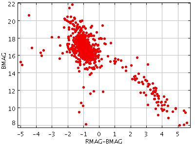
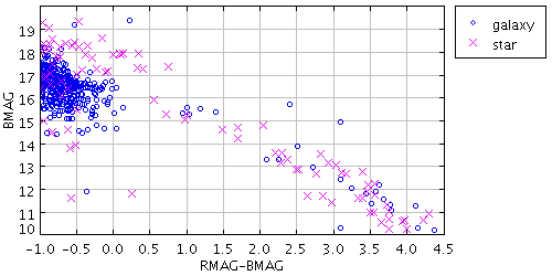
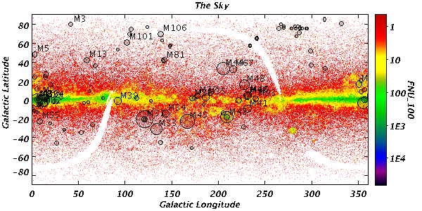
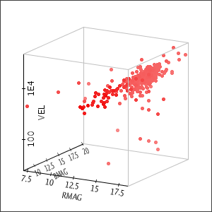
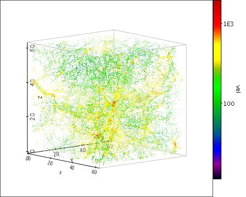
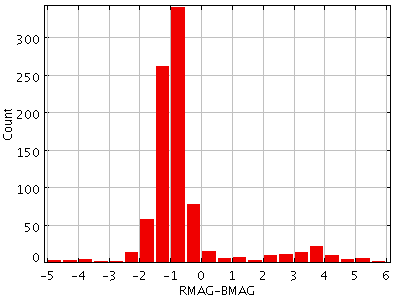
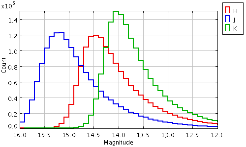