Next Previous Up Contents
Next: Shading Modes
Up: Plot Forms
Previous: StatMark Form
The ArrayQuantile form ( ),
available from the
XYArray Layer Control,
displays a quantile or quantile range for a set of plotted X/Y array pairs.
If a table contains one spectrum per row in array-valued wavelength
and flux columns, this plotter can be used to display a median of all
the spectra, or a range between two quantiles. Smoothing options are
available to even out noise arising from the pixel binning.
),
available from the
XYArray Layer Control,
displays a quantile or quantile range for a set of plotted X/Y array pairs.
If a table contains one spectrum per row in array-valued wavelength
and flux columns, this plotter can be used to display a median of all
the spectra, or a range between two quantiles. Smoothing options are
available to even out noise arising from the pixel binning.
For each row, the X Values and Y Values
arrays must be the same length as each other,
but this plot type does not
(unlike StatMark and
StatLine)
require the arrays to be sampled into the same bins for each row.
The algorithm calculates quantiles for all the X,Y points plotted in
each column of pixels. This means that more densely sampled spectra have
more influence on the output than sparser ones.
Note:
In the current implementation, depending on the details of the
configuration and the data, there may be some distortions or missing
graphics near the edges of the plot.
This may be improved in future releases, depending on feedback.
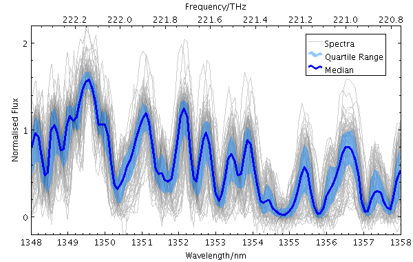
Example ArrayQuantile plot
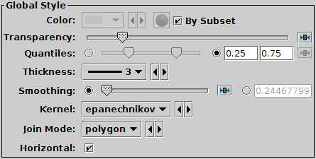
ArrayQuantile form configuration panel
The configuration options are:
-
Transparency
- Transparency with which components are plotted,
from opaque to invisible.
-
Quantiles
- Defines the quantile or quantile range of values that should be
marked in each pixel column (or row).
The slider control goes from 0 (minimum in pixel column/row)
to 1 (maximum in pixel column/row), so 0.5 indicates the median.
This control is a double-slider, so you can drag out a range
of values. If the values are the same as each other, a single
point will be indicated, but if there is a range then the area
between the indicated quantiles will be filled.
The radio buttons let you toggle between using the slider to
set the quantile value(s) or entering them in the text fields.
If the two values are identical, you can leave the second text field blank.
-
Thickness
- Sets the minimum extent of the markers that are plotted in each
pixel column (or row) to indicate the designated value range. If the
range is zero sized (two bounding quantiles are equal)
this will give the actual thickness of the plotted line.
If the range is non-zero however, the line may be thicker than this in
places according to the quantile positions.
-
Smoothing
- Configures the smoothing width.
This is the characteristic width of the Kernel
function to be convolved with the density in one dimension
to smooth the quantile function.
You can adjust it using the slider (wider smoothing to the right)
or enter a value in data coordinates explicitly in the text field.
If the smoothed axis is logarithmic, the value is a multiplication factor
rather than an additive increment.
-
Kernel
- The functional form of the smoothing kernel. The functions listed
refer to the unscaled shape; all kernels are normalised to give a
total area of unity.
The available options are:
-
square:
Uniform value: f(x)=1, |x|=0..1
-
linear:
Triangle: f(x)=1-|x|, |x|=0..1
-
epanechnikov:
Parabola: f(x)=1-x*x, |x|=0..1
-
cos:
Cosine: f(x)=cos(x*pi/2), |x|=0..1
-
cos2:
Cosine squared: f(x)=cos^2(x*pi/2), |x|=0..1
-
gauss3: Gaussian truncated at 3.0 sigma:
f(x)=exp(-x*x/2), |x|=0..3
-
gauss6: Gaussian truncated at 6.0 sigma:
f(x)=exp(-x*x/2), |x|=0..6
-
Join Mode
- Defines the graphical style for connecting distinct quantile values.
If smoothed samples are packed more closely than the pixel grid
the option chosen here doesn't make much difference,
but if there are gaps in the data along the sampled axis,
it's useful to have a guide to the eye to join one quantile
determination to the next.
The available options are:
-
none:
displayed quantile ranges are not joined
-
polygon:
the area between a line connecting the upper quantiles
and a line connecting the lower quantiles is filled
-
lines:
a line of thickness given by Thickness
is drawn from the center of each quantile range to the next
-
Horizontal
- Determines whether the trace bins are horizontal or vertical.
If true, y quantiles are calculated for each pixel column,
and if false, x quantiles are calculated for each pixel row.
Next Previous Up Contents
Next: Shading Modes
Up: Plot Forms
Previous: StatMark Form
TOPCAT - Tool for OPerations on Catalogues And Tables
Starlink User Note253
TOPCAT web page:
http://www.starlink.ac.uk/topcat/
Author email:
m.b.taylor@bristol.ac.uk
Mailing list:
topcat-user@jiscmail.ac.uk