Starlink User Note 253
Mark Taylor
14 May 2026
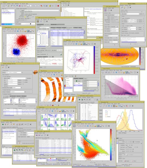
TOPCAT is an interactive graphical viewer and editor for tabular data. It has been designed for use with astronomical tables such as object catalogues, but is not restricted to astronomical applications. It understands a number of different astronomically important formats, and more formats can be added. It is designed to cope well with large tables; a million rows by a hundred columns should not present a problem even with modest memory and CPU resources.
It offers a variety of ways to view and analyse the data, including a browser for the cell data themselves, viewers for information about table and column metadata, tools for joining tables using flexible matching algorithms, and extensive 2- and 3-d visualisation facilities. Using a powerful and extensible Java-based expression language new columns can be defined and row subsets selected for separate analysis. Selecting a row can be configured to trigger an action, for instance displaying an image of the catalogue object in an external viewer. Table data and metadata can be edited and the resulting modified table can be written out in a wide range of output formats.
A number of options are provided for loading data from external sources, including Virtual Observatory (VO) services, thus providing a gateway to many remote archives of astronomical data. It can also interoperate with other desktop tools using the SAMP protocol.
TOPCAT is written in pure Java (except for a few optional libraries) and is available under the GNU General Public Licence. Its underlying table processing facilities are provided by STIL, the Starlink Tables Infrastructure Library.
TOPCAT is an interactive graphical program which can examine, analyse, combine, edit and write out tables. A table is, roughly, something with columns and rows; each column contains objects of the same type (for instance floating point numbers) and each row has an entry for each of the columns (though some entries might be blank). A common astronomical example of a table is an object catalogue.
TOPCAT can read in tables in a number of formats from various sources, allow you to inspect and manipulate them in various ways, and if you have edited them optionally write them out in the modified state for later use, again in a variety of formats. Here is a summary of its main capabilities:
Considerable effort has gone into making it work with large tables; a few million rows and hundreds of columns is usually quite manageable.
The general idea of the program is quite straightforward. At any time, it has a list of tables it knows about - these are displayed in the Control Window which is the first thing you see when you start up the program. You can add to the list by loading tables in, or by some actions which create new tables from the existing ones. When you select a table in the list by clicking on it, you can see general information about it in the control window, and you can also open more specialised view windows which allow you to inspect it in more detail or edit it. Some of the actions you can take, such as changing the current Sort Order, Row Subset or Column Set change the Apparent Table, which is a view of the table used for things such as saving it and performing row matches. Changes that you make do not directly modify the tables on disk (or wherever they came from), but if you want to save the changes you have made, you can write the modified table(s) to a new location.
The main body of this document explains these ideas and capabilities
in more detail, and
Appendix A gives a full description of all the windows which
form the application.
While the program is running, this document is available via the
online help system - clicking the Help ( )
toolbar button in any window will pop up a help browser open at
the page which describes that window.
This document is heavily hyperlinked, so you may find it easier to
read in its HTML form than on paper.
)
toolbar button in any window will pop up a help browser open at
the page which describes that window.
This document is heavily hyperlinked, so you may find it easier to
read in its HTML form than on paper.
Recent news about the program can be found on the TOPCAT web page. It was initially developed within the now-terminated Starlink and then AstroGrid projects, and has subsequently been supported by the UK's PPARC and STFC research councils, various Euro-VO and FP7 projects, GAVO and ESA. The underlying table handling facilities are supplied by the Starlink Tables Infrastructure Library STIL, which is documented more fully in SUN/252. The software is written in pure Java (except for some compression codecs used by the Parquet I/O handlers), and should run on any J2SE platform version 1.8 or later. This makes it highly portable, since it can run on any machine which has a suitable Java installation, which is available for MS Windows, Mac OS X and most flavours of Unix amongst others. Some of the external viewer applications it talks to rely on non-Java code however so one or two facilities, such as displaying spectra, may be absent in some cases.
The TOPCAT application is available under the terms of the GNU General Public License, since some of the libraries it uses are also GPL. However, all of the original code and many of the libraries it uses may alternatively be used under more permissive licenses such as the GNU Lesser General Public License, see documentation of the STILTS package for more details.
This manual aims to give detailed tutorial and reference documentation on most aspects of TOPCAT's capabilities, and reading it is an excellent way to learn about the program. However, it's quite a fat document, and if you feel you've got better things to do with your time than read it all, you should be able to do most things by playing around with the software and dipping into the manual (or equivalently the online help) when you can't see how to do something or the program isn't behaving as expected. This section provides a short introduction for the impatient, explaining how to get started.
To start the program, you will probably type topcat or
something like
java -jar topcat-full.jar (see Section 10 for
more detail). To view a table that you have on disk, you can either
give its name on the command line or load it using the Load
button from the GUI.
FITS, VOTable, ECSV, CDF, PDS4, feather, Parquet and GBIN files
are recognised automatically;
if your data is in another format such as ASCII (see Section 4.1.1)
you need to tell the program (e.g. -f ascii on the command line).
If you just want to try the program out, topcat -demo will
start with a couple of small tables for demonstration purposes.
The first thing that you see is the Control Window. This has a list of the loaded table(s) on the left. If one of these is highlighted by clicking on it, information about it will be shown on the right; some of this (table name, sort order) you can change here. Along the top is a toolbar with a number of buttons, most of which open up new windows. These correspond to some of the things you might most often want to do in TOPCAT, and fall into a few groups:


The menus provide alternative ways to open up these windows,
and also list a number of other, less commonly-used, options.
The Help () button appears in most windows -
if you click it a help browser will be displayed showing an appropriate
part of this manual.
The Help menu gives you a few
more options along the same lines, including displaying the help
information in your usual web browser rather than in TOPCAT's (somewhat
scrappy) help viewer.
All the windows follow roughly this pattern. For some of the toolbar
buttons you can probably guess what they do from their icons,
for others probably not - to find out
you can hover with the mouse to see the tooltip,
look in the menus, read the manual, or just push it and see.
Some of the windows allow you to make changes of various sorts to the tables, such as performing sorts, selecting rows, modifying data or metadata. None of these affect the table on disk (or database, or wherever), but if you subsequently save the table the changes will be reflected in the table that you save.
A notable point to bear in mind concerns memory.
TOPCAT is fairly efficient in use of memory, but in some cases when
dealing with large tables you might see an OutOfMemoryError.
It is usually possible to work round this by using the
-XmxNNNM
flag on startup - see Section 10.2.2.
Finally, if you have queries, comments or requests about the software, and they don't appear to be addressed in the manual, consult the TOPCAT web page, use the topcat-user mailing list, or contact the author - user feedback is always welcome.
The Apparent Table is a particular view of a table which can be influenced by some of the viewing controls.
When you load a table into TOPCAT it has a number of characteristics like the number of columns and rows it contains, the order of the rows that make up the data, the data and metadata themselves, and so on. While manipulating it you can modify the way that the table appears to the program, by changing or adding data or metadata, or changing the order or selection of columns or rows that are visible. For each table its "apparent table" is a table which corresponds to the current state of the table according to the changes that you have made.
In detail, the apparent table consists of the table as it was originally imported into the program plus any of the following changes that you have made:
The apparent table is used in the following contexts:
 ) toolbar button,
the resulting table will contain only those ten rows.
) toolbar button,
the resulting table will contain only those ten rows.
An important feature of TOPCAT is the ability to define and use Row Subsets. A Row Subset is a selection of the rows within a whole table being viewed within the application, or equivalently a new table composed from some subset of its rows. You can define these and use them in several different ways; the usefulness comes from defining them in one context and using them in another. The Subset Window displays the currently defined Row Subsets and permits some operations on them.
At any time each table has a current row subset, and this affects the Apparent Table. You can always see what it is by looking at the "Row Subset" selector in the Control Window when that table is selected; by default it is one containing all the rows. You can change it by choosing from this selector or as a result of some other actions.
Other contexts in which subsets can be used are picking a selection of rows from which to calculate in the Statistics Window and marking groups of rows to plot using different markers in the various plotting (and old-style plotting) windows.
Tables always have two special subsets:
You can define a Row Subset in one of the following ways:
 ) button will pop up
the Algebraic Subset Window
which allows you to define a new subset using an algebraic expression
based on the values of the cells in each row.
The format of such expressions is described in Section 7.
The Subsets Window also provides some variants on this option
for convenience, like selecting
the first N (
) button will pop up
the Algebraic Subset Window
which allows you to define a new subset using an algebraic expression
based on the values of the cells in each row.
The format of such expressions is described in Section 7.
The Subsets Window also provides some variants on this option
for convenience, like selecting
the first N ( ),
last N (
),
last N ( ),
or every Nth (
),
or every Nth ( ) rows,
or the complement (
) rows,
or the complement ( ) of an existing subset.
 ),
Algebraic Subset From Visible (
),
Algebraic Subset From Visible ( ),
Draw Subset Blob (
),
Draw Subset Blob ( ) and
Draw Algebraic Subset (
) and
Draw Algebraic Subset ( ),
though not all are available for all plot types.
),
though not all are available for all plot types.
 ) or
Subset From Unselected Rows (
) or
Subset From Unselected Rows ( )
buttons to create a new subset based
on the set of highlighted rows or their complement.
Combining this with sorting
the rows in the table can be useful;
if you do a Sort Up on a given column and then drag out the
top few rows of the table you can easily create a subset consisting
of the highest values of a given column.
)
buttons to create a new subset based
on the set of highlighted rows or their complement.
Combining this with sorting
the rows in the table can be useful;
if you do a Sort Up on a given column and then drag out the
top few rows of the table you can easily create a subset consisting
of the highest values of a given column.
In all these cases you will be asked to assign a name for the subset. As with column names, it is a good idea to follow a few rules for these names so that they can be used in algebraic expressions. They should be:
In the first subset definition method above, the current subset will be set immediately to the newly created one. In other cases the new subset may be highlighted appropriately in other windows, for instance by being plotted in scatter plot windows.
You can sort the rows of each table according to the values in the table. Normally you will want to sort on a numeric column, but other values may be sortable too, for instance a String column will sort alphabetically. Some kinds of columns (e.g. array ones) don't have any well-defined order, and it is not possible to select these for sorting on.
At any time, each table has a current row order,
and this affects the Apparent Table.
You can always see what it is by looking under
the Sort Order item
in the Control Window when that table
is selected; by default it is blank, which means the rows have the
same order as that of the table they were loaded in from.
The little arrow (![]() /
/![]() ) indicates whether
the sense of the sort is up or down.
You can change the sort order by selecting a column name
or entering an algebraic expression
in this selector, and change the sense by clicking on the arrow.
To sort on multiple columns, use the Add/Remove Selector
(
) indicates whether
the sense of the sort is up or down.
You can change the sort order by selecting a column name
or entering an algebraic expression
in this selector, and change the sense by clicking on the arrow.
To sort on multiple columns, use the Add/Remove Selector
( ) buttons to change the number of selectors;
selectors to the left are more significant, and ones to the right
are used in case of a tie in earlier values.
The sort order can also be changed by using menu items in the
Columns Window or right-clicking
popup menus in the Data Window.
) buttons to change the number of selectors;
selectors to the left are more significant, and ones to the right
are used in case of a tie in earlier values.
The sort order can also be changed by using menu items in the
Columns Window or right-clicking
popup menus in the Data Window.
Selecting values to sort by calculates the new row order by performing a sort on the cell values there and then. If the table data change somehow (e.g. because you edit cells in the table) then it is possible for the sort order to become out of date. If that happens you can resort by making a new selection and then changing it back again.
The current row order affects the Apparent Table, and hence determines the order of rows in tables which are exported in any way (e.g. written out) from TOPCAT. You can always see the rows in their currently sorted order in the Data Window.
When each table is imported it has a list of columns. Each column has header information which determines the kind of data which can fill the cells of that column as well as a name, and maybe some additional information like units and Unified Content Descriptor. All this information can be viewed, and in some cases modified, in the Columns Window.
During the lifetime of the table within TOPCAT, this list of columns can be changed by adding new columns, hiding (and perhaps subsequently revealing) existing columns, and changing their order. The current state of which columns are present and visible and what order they are in is collectively known as the Column Set, and affects the Apparent Table. The current Column Set is always reflected in the columns displayed in the Data Window and Statistics Window. The Columns Window shows all the known columns, including hidden ones; whether they are currently visible is indicated by the checkbox in the Visible column. By default, the Columns Window and Statistics Window also reflect the current column set order, though there are options to change this view.
You can affect the current Column Set in the following ways:
 ) or
Reveal Selected (
) or
Reveal Selected ( )
button in the toolbar or menu.
Note when selecting rows, don't drag the mouse over the Visible
column, do it somewhere in the middle of the table.
The Hide All (
)
button in the toolbar or menu.
Note when selecting rows, don't drag the mouse over the Visible
column, do it somewhere in the middle of the table.
The Hide All ( ) and
Reveal All (
) and
Reveal All ( )
buttons set all columns in the table invisible or visible -
a useful convenience if you've got a very wide table.
)
buttons set all columns in the table invisible or visible -
a useful convenience if you've got a very wide table.
You can also hide a column by right-clicking on it in the Data Window, which brings up a popup menu - select the Hide option. To make it visible again you have to go to the Columns Window as above.
)
or New Sky Coordinate Columns ( ) buttons in the
Columns Window or the (right-click) popup menu in the
Data Window to add new columns derived from exsiting ones.
) buttons in the
Columns Window or the (right-click) popup menu in the
Data Window to add new columns derived from exsiting ones.
 ) button.
This is similar to the Add a Synthetic Column
described in the previous item, but it pops up a new column
dialogue with similar characteristics (name, units etc)
to those of the column that's being replaced, and when completed
it slots the new column in to the table hiding the old one.
) button.
This is similar to the Add a Synthetic Column
described in the previous item, but it pops up a new column
dialogue with similar characteristics (name, units etc)
to those of the column that's being replaced, and when completed
it slots the new column in to the table hiding the old one.
 ) button, which will add
a new boolean column to the table with the value true
for rows part of that subset and false for the other rows.
) button, which will add
a new boolean column to the table with the value true
for rows part of that subset and false for the other rows.
Tables can be loaded into TOPCAT using the Load Window or from the command line, or acquired from VO services, and saved using the Save Window. This section describes the file formats supported for input and output, as well as the syntax to use when specifying a table by name, either as a file/URL or using a scheme specification.
TOPCAT supports a number of different serialization formats for table data; some have better facilities for storing table data and metadata than others.
Since you can load a table from one format and save it in a different
one, TOPCAT can be used to convert a table from one format to another.
If this is all you want to do however, you may find it more
convenient to use the tcopy or tpipe
command line utilities in the
STILTS package.
The following subsections describe the available formats for reading and writing tables. The two operations are separate, so not all the supported input formats have matching output formats and vice versa.
Loading table into TOPCAT from files or URLs is done either
using the Load Table dialogue
or one of its sub-windows,
or from the command line when you start the program.
For some file formats (e.g. FITS, VOTable, CDF),
the format can be automatically determined by
looking at the file content, regardless of filename;
for others (e.g. CSV files with a ".csv" extension),
TOPCAT may be able to use the filename as a hint to guess the format
(the details of these rules are given in the format-specific
subsections below).
In other cases though,
you will have to specify the format that the file is in.
In the Load Window, there is a selection box from which you can
choose the format, and from the command line you use the
-f flag - see Section 10 for details.
You can always specify the format rather than using automatic detection
if you prefer - this is slightly more efficient,
and may give you a more detailed error message
if a table fails to load.
In either case, table locations may be given as filenames or as URLs, and any data compression (gzip, unix compress and bzip2) will be automatically detected and dealt with - see Section 4.2.
Some of the formats
(e.g. FITS, VOTable)
are capable of storing more than one table;
usually loading such files loads all the tables into TOPCAT.
If you want to specify only a single table,
you can give a position indicator either after a "#" sign
at the end of the filename or using the
Position in file field in the
Filestore Browser or similar.
The details of the syntax for this is given in the relevant
format description below.
The following sections describe the table formats which TOPCAT can read.
FITS is a very well-established format for storage of
astronomical table or image data
(see https://fits.gsfc.nasa.gov/).
This reader can read tables stored in
binary (XTENSION='BINTABLE') and
ASCII (XTENSION='TABLE') table extensions;
any image data is ignored.
Currently, binary table extensions are read much more efficiently
than ASCII ones.
When a table is stored in a BINTABLE extension in an uncompressed FITS file on disk, the table is 'mapped' into memory; this generally means very fast loading and low memory usage. FITS tables are thus usually efficient to use.
Limited support is provided for the semi-standard HEALPix-FITS convention; such information about HEALPix level and coordinate system is read and made available for application usage and user examination.
A private convention is used to support encoding of tables with more than 999 columns (not possible in standard FITS); see Section 4.1.3.2.
Header cards in the table's HDU header will be made available as table parameters. Only header cards which are not used to specify the table format itself are visible as parameters (e.g. NAXIS, TTYPE* etc cards are not). HISTORY and COMMENT cards are run together as one multi-line value.
Any 64-bit integer column with a non-zero integer offset
(TFORMn='K', TSCALn=1, TZEROn<>0)
is represented in the read table as Strings giving the decimal integer value,
since no numeric type in Java is capable of representing the whole range of
possible inputs. Such columns are most commonly seen representing
unsigned long values.
Where a multi-extension FITS file contains more than one table, a single table may be specified using the position indicator, which may take one of the following forms:
spec23.fits.gz"
with one primary HDU and two BINTABLE extensions,
you would view the first one using the name "spec23.fits.gz"
or "spec23.fits.gz#1"
and the second one using the name "spec23.fits.gz#2".
The suffix "#0" is never used for a legal
FITS file, since the primary HDU cannot contain a table.
EXTNAME header in the HDU,
or alternatively the value of EXTNAME
followed by "-" followed by the value of EXTVER.
This follows the recommendation in
the FITS standard that EXTNAME and EXTVER
headers can be used to identify an HDU.
So in a multi-extension FITS file "cat.fits"
where a table extension
has EXTNAME='UV_DATA' and EXTVER=3,
it could be referenced as
"cat.fits#UV_DATA" or "cat.fits#UV_DATA-3".
Matching of these names is case-insensitive.
Files in this format may contain multiple tables;
depending on the context, either one or all tables
will be read.
Where only one table is required,
either the first one in the file is used,
or the required one can be specified after the
"#" character at the end of the filename.
This format can be automatically identified by its content so you do not need to specify the format explicitly when reading FITS tables, regardless of the filename.
There are actually two FITS input handlers,
fits-basic and fits-plus.
The fits-basic handler extracts standard column metadata
from FITS headers of the HDU in which the table is found,
while the fits-plus handler reads column and table metadata
from VOTable content stored in the primary HDU of the multi-extension
FITS file.
FITS-plus is a private convention effectively defined by the
corresponding output handler; it allows de/serialization of
much richer metadata than can be stored in standard FITS headers
when the FITS file is read by fits-plus-aware readers,
though other readers can understand the unenhanced FITS file perfectly well.
It is normally not necessary to worry about this distinction;
TOPCAT will determine whether a FITS file is FITS-plus or not based on its
content and use the appropriate handler, but if you want to force the
reader to use or ignore the enriched header, you can explicitly select
an input format of "FITS-plus" or "FITS".
The details of the FITS-plus convention are described in Section 4.1.3.1.
As well as normal binary and ASCII FITS tables, STIL supports
FITS files which contain tabular data stored in column-oriented format.
This means that the table is stored in a BINTABLE extension HDU,
but that BINTABLE has a single row, with each cell of that row
holding a whole column's worth of data. The final (slowest-varying)
dimension of each of these cells (declared via the TDIMn headers)
is the same for every column, namely,
the number of rows in the table that is represented.
The point of this is that all the cells for each column are stored
contiguously, which for very large, and especially very wide tables
means that certain access patterns (basically, ones which access
only a small proportion of the columns in a table) can be much more
efficient since they require less I/O overhead in reading data blocks.
Such tables are perfectly legal FITS files, but general-purpose FITS software may not recognise them as multi-row tables in the usual way. This format is mostly intended for the case where you have a large table in some other format (possibly the result of an SQL query) and you wish to cache it in a way which can be read efficiently by a STIL-based application.
For performance reasons, it is advisable to access colfits files uncompressed on disk. Reading them from a remote URL, or in gzipped form, may be rather slow (in earlier versions it was not supported at all).
This format can be automatically identified by its content so you do not need to specify the format explicitly when reading colfits-basic tables, regardless of the filename.
Like the normal (row-oriented) FITS handler,
two variants are supported:
with (colfits-plus) or without (colfits-basic)
metadata stored as a VOTable byte array in the primary HDU.
For details of the FITS-plus convention, see Section 4.1.3.1.
VOTable is an XML-based format for tabular data endorsed by the International Virtual Observatory Alliance; while the tabular data which can be encoded is by design close to what FITS allows, it provides for much richer encoding of structure and metadata. Most of the table data exchanged by VO services is in VOTable format, and it can be used for local table storage as well.
Any table which conforms to the VOTable 1.0, 1.1, 1.2, 1.3 or 1.4 specifications can be read. This includes all the defined cell data serializations; cell data may be included in-line as XML elements (TABLEDATA serialization), included/referenced as a FITS table (FITS serialization), or included/referenced as a raw binary stream (BINARY or BINARY2 serialization). The handler does not attempt to be fussy about input VOTable documents, and it will have a good go at reading VOTables which violate the standards in various ways.
Much, but not all, of the metadata contained in a VOTable
document is retained when the table is read in.
The attributes
unit, ucd, xtype and utype,
and the elements
COOSYS, TIMESYS and DESCRIPTION
attached to table columns or parameters,
are read and may be used by the application as appropriate
or examined by the user.
However, information encoded in the hierarchical structure
of the VOTable document, including GROUP structure, is not
currently retained when a VOTable is read.
VOTable documents may contain more than one actual table
(TABLE element).
To specify a specific single table,
the table position indicator is given by the
zero-based index of the TABLE element in a breadth-first search.
Here is an example VOTable document:
   <VOTABLE>
     <RESOURCE>
       <TABLE name="Star Catalogue"> ... </TABLE>
       <TABLE name="Galaxy Catalogue"> ... </TABLE>
     </RESOURCE>
   </VOTABLE>
If this is available in a file named "cats.xml"
then the two tables could be named as
"cats.xml#0" and "cats.xml#1" respectively.
Files in this format may contain multiple tables;
depending on the context, either one or all tables
will be read.
Where only one table is required,
either the first one in the file is used,
or the required one can be specified after the
"#" character at the end of the filename.
This format can be automatically identified by its content so you do not need to specify the format explicitly when reading VOTable tables, regardless of the filename.
NASA's Common Data Format, described at https://cdf.gsfc.nasa.gov/, is a binary format for storing self-described data. It is typically used to store tabular data for subject areas like space and solar physics.
CDF does not store tables as such, but sets of variables
(columns) which are typically linked to a time quantity;
there may be multiple such disjoint sets in a single CDF file.
This reader attempts to extract these sets into separate tables
using, where present, the DEPEND_0 attribute
defined by the
ISTP Metadata Guidelines.
Where there are multiple tables they can be identified
using a "#" symbol at the end of the filename
by index ("<file>.cdf#0" is the first table)
or by the name of the independent variable
("<file>.cdf#EPOCH" is the table relating to
the EPOCH column).
Files in this format may contain multiple tables;
depending on the context, either one or all tables
will be read.
Where only one table is required,
either the first one in the file is used,
or the required one can be specified after the
"#" character at the end of the filename.
This format can be automatically identified by its content so you do not need to specify the format explicitly when reading CDF tables, regardless of the filename.
Comma-separated value ("CSV") format is a common semi-standard text-based format in which fields are delimited by commas. Spreadsheets and databases are often able to export data in some variant of it. The intention is to read tables in the version of the format spoken by MS Excel amongst other applications, though the documentation on which it was based was not obtained directly from Microsoft.
The rules for data which it understands are as follows:
#" character
(or anything else) to introduce "comment" lines.
Because the CSV format contains no metadata beyond column names,
the handler is forced to guess the datatype of the values in each column.
It does this by reading the whole file through once and guessing
on the basis of what it has seen (though see the maxSample
configuration option). This has the disadvantages:
The delimiter option makes it possible to use non-comma
characters to separate fields. Depending on the character used this
may behave in surprising ways; in particular for space-separated fields
the ascii format may be a better choice.
The handler behaviour may be modified by specifying
one or more comma-separated name=value configuration options
in parentheses after the handler name, e.g.
"csv(header=true,delimiter=|)".
The following options are available:
header = true|false|null
true: the first line is a header line containing column namesfalse: all lines are data lines, and column names will be assigned automaticallynull: a guess will be made about whether the first line is a header or not depending on what it looks likenull (auto-determination).
This usually works OK, but can get into trouble if
all the columns look like string values.
(Default: null)
delimiter = <char>|0xNN
|", a hexadecimal character code like "0x7C", or one of the names "comma", "space" or "tab". Some choices of delimiter, for instance whitespace characters, might not work well or might behave in surprising ways.
(Default: ,)
maxSample = <int>
0)
notypes = <type>[;<type>...]
blank, boolean, short, int, long, float, double, date, hms and dms. So if you want to make sure that all integer and floating-point columns are 64-bit (i.e. long and double respectively) you can set this value to "short;int;float".encoding = ASCII|UTF-8|UTF-16|...
UTF-8)
This format cannot be automatically identified
by its content, so in general it is necessary
to specify that a table is in
CSV
format when reading it.
However, if the input file has
the extension ".csv" (case insensitive)
an attempt will be made to read it using this format.
An example looks like this:
RECNO,SPECIES,NAME,LEGS,HEIGHT,MAMMAL
1,pig,Pigling Bland,4,0.8,true
2,cow,Daisy,4,2.0,true
3,goldfish,Dobbin,,0.05,false
4,ant,,6,0.001,false
5,ant,,6,0.001,false
6,queen ant,Ma'am,6,0.002,false
7,human,Mark,2,1.8,true
See also ECSV as a format which is similar and capable of storing more metadata.
The Enhanced Character Separated Values format was developed within the Astropy project and is described in Astropy APE6 (DOI). It is composed of a YAML header followed by a CSV-like body, and is intended to be a human-readable and maybe even human-writable format with rich metadata. Most of the useful per-column and per-table metadata is preserved when de/serializing to this format. The version supported by this reader is currently ECSV 1.0.
There are various ways to format the YAML header, but a simple example of an ECSV file looks like this:
# %ECSV 1.0
# ---
# delimiter: ','
# datatype: [
#   { name: index,   datatype: int32   },
#   { name: Species, datatype: string  },
#   { name: Name,    datatype: string  },
#   { name: Legs,    datatype: int32   },
#   { name: Height,  datatype: float64, unit: m },
#   { name: Mammal,  datatype: bool    },
# ]
index,Species,Name,Legs,Height,Mammal
1,pig,Bland,4,,True
2,cow,Daisy,4,2,True
3,goldfish,Dobbin,,0.05,False
4,ant,,6,0.001,False
5,ant,,6,0.001,False
6,human,Mark,2,1.9,True
If you follow this pattern, it's possible to write your own ECSV files by
taking an existing CSV file
and decorating it with a header that gives column datatypes,
and possibly other metadata such as units.
This allows you to force the datatype of given columns
(the CSV reader guesses datatype based on content, but can get it wrong)
and it can also be read much more efficiently than a CSV file
and its format can be detected automatically.
The header information can be provided either in the ECSV file itself,
or alongside a plain CSV file from a separate source
referenced using the header configuration option.
In Gaia EDR3 for instance, the ECSV headers are supplied alongside
the CSV files available for raw download of all tables in the
Gaia source catalogue, so e.g. STILTS can read
one of the gaia_source CSV files with full metadata
as follows:
   stilts tpipe
      ifmt='ecsv(header=http://cdn.gea.esac.esa.int/Gaia/gedr3/ECSV_headers/gaia_source.header)'
      in=http://cdn.gea.esac.esa.int/Gaia/gedr3/gaia_source/GaiaSource_000000-003111.csv.gz
The ECSV datatypes that work well with this reader are
bool,
int8, int16, int32, int64,
float32, float64
and
string.
Array-valued columns are also supported with some restrictions.
Following the ECSV 1.0 specification,
columns representing arrays of the supported datatypes can be read,
as columns with datatype: string and a suitable
subtype, e.g.
"int32[<dims>]" or "float64[<dims>]".
Fixed-length arrays (e.g. subtype: int32[3,10])
and 1-dimensional variable-length arrays
(e.g. subtype: float64[null]) are supported;
however variable-length arrays with more than one dimension
(e.g. subtype: int32[4,null]) cannot be represented,
and are read in as string values.
Null elements of array-valued cells are not supported;
they are read as NaNs for floating point data, and as zero/false for
integer/boolean data.
ECSV 1.0, required to work with array-valued columns,
is supported by Astropy v4.3 and later.
The handler behaviour may be modified by specifying
one or more comma-separated name=value configuration options
in parentheses after the handler name, e.g.
"ecsv(header=http://cdn.gea.esac.esa.int/Gaia/gedr3/ECSV_headers/gaia_source.header,colcheck=FAIL)".
The following options are available:
header = <filename-or-url>
null)
colcheck = IGNORE|WARN|FAIL
WARN)
This format can be automatically identified by its content so you do not need to specify the format explicitly when reading ECSV tables, regardless of the filename.
In many cases tables are stored in some sort of unstructured plain text format, with cells separated by spaces or some other delimiters. There is a wide variety of such formats depending on what delimiters are used, how columns are identified, whether blank values are permitted and so on. It is impossible to cope with them all, but the ASCII handler attempts to make a good guess about how to interpret a given ASCII file as a table, which in many cases is successful. In particular, if you just have columns of numbers separated by something that looks like spaces, you should be just fine.
Despite the name, by default it reads Unicode characters in the UTF-8
encoding. It can if necessary be restricted to ASCII characters only
by setting the encoding option.
Here are the detailed rules for how the ASCII-format tables are interpreted:
null" (unquoted) represents
the null valueBoolean,
Short
Integer,
Long,
Float,
Double,
String
NaN for not-a-number, which is treated the same as a
null value for most purposes, and Infinity or inf
for infinity (with or without a preceding +/- sign).
These values are matched case-insensitively.If the list of rules above looks frightening, don't worry, in many cases it ought to make sense of a table without you having to read the small print. Here is an example of a suitable ASCII-format table:
    #
    # Here is a list of some animals.
    #
    # RECNO  SPECIES         NAME         LEGS   HEIGHT/m
      1      pig             "Pigling Bland"  4  0.8
      2      cow             Daisy        4      2
      3      goldfish        Dobbin       ""     0.05
      4      ant             ""           6      0.001
      5      ant             ""           6      0.001
      6      ant             ''           6      0.001
      7      "queen ant"     'Ma\'am'     6      2e-3
      8      human           "Mark"       2      1.8
In this case it will identify the following columns:
    Name       Type
    ----       ----
    RECNO      Short
    SPECIES    String
    NAME       String
    LEGS       Short
    HEIGHT/m   Float
It will also use the text "Here is a list of some animals"
as the Description parameter of the table.
Without any of the comment lines, it would still interpret the table,
but the columns would be given the names col1..col5.
The handler behaviour may be modified by specifying
one or more comma-separated name=value configuration options
in parentheses after the handler name, e.g.
"ascii(maxSample=100000,notypes=short;float)".
The following options are available:
maxSample = <int>
0)
notypes = <type>[;<type>...]
blank, boolean, short, int, long, float, double, date, hms and dms. So if you want to make sure that all integer and floating-point columns are 64-bit (i.e. long and double respectively) you can set this value to "short;int;float".encoding = ASCII|UTF-8|UTF-16|...
UTF-8)
This format cannot be automatically identified
by its content, so in general it is necessary
to specify that a table is in
ASCII
format when reading it.
However, if the input file has
the extension ".txt" (case insensitive)
an attempt will be made to read it using this format.
CalTech's Infrared Processing and Analysis Center use a text-based format for storage of tabular data, defined at http://irsa.ipac.caltech.edu/applications/DDGEN/Doc/ipac_tbl.html. Tables can store column name, type, units and null values, as well as table parameters.
This format cannot be automatically identified
by its content, so in general it is necessary
to specify that a table is in
IPAC
format when reading it.
However, if the input file has
the extension ".tbl" or ".ipac" (case insensitive)
an attempt will be made to read it using this format.
An example looks like this:
\Table name = "animals.vot"
\Description = "Some animals"
\Author = "Mark Taylor"
| RECNO | SPECIES   | NAME          | LEGS | HEIGHT | MAMMAL |
| int   | char      | char          | int  | double | char   |
|       |           |               |      | m      |        |
| null  | null      | null          | null | null   | null   |
  1       pig         Pigling Bland   4      0.8      true
  2       cow         Daisy           4      2.0      true
  3       goldfish    Dobbin          null   0.05     false
  4       ant         null            6      0.001    false
  5       ant         null            6      0.001    false
  6       queen ant   Ma'am           6      0.002    false
  7       human       Mark            2      1.8      true
NASA's Planetary Data System version 4 format is described at https://pds.nasa.gov/datastandards/. This implementation is based on v1.16.0 of PDS4.
PDS4 files consist of an XML Label file which
provides detailed metadata, and which may also contain references
to external data files stored alongside it.
This input handler looks for (binary, character or delimited)
tables in the Label;
depending on the configuration it may restrict them to those
in the File_Area_Observational area.
The Label is the file which has to be presented to this
input handler to read the table data.
Because of the relationship between the label and the data files,
it is usually necessary to move them around together.
If there are multiple tables in the label,
you can refer to an individual one using the "#"
specifier after the label file name by table name,
local_identifier, or 1-based index
(e.g. "label.xml#1" refers to the first table).
If there are Special_Constants defined
in the label, they are in most cases interpreted as blank values
in the output table data.
At present, the following special values are interpreted
as blanks:
saturated_constant,
missing_constant,
error_constant,
invalid_constant,
unknown_constant,
not_applicable_constant,
high_instrument_saturation,
high_representation_saturation,
low_instrument_saturation,
low_representation_saturation
.
Fields within top-level Groups are interpreted as array values. Any fields in nested groups are ignored. For these array values only limited null-value substitution can be done (since array elements are primitives and so cannot take null values).
This input handler is somewhat experimental, and the author is not a PDS expert. If it behaves strangely or you have suggestions for how it could work better, please contact the author.
The handler behaviour may be modified by specifying
one or more comma-separated name=value configuration options
in parentheses after the handler name, e.g.
"pds4(checkmagic=false,observational=true)".
The following options are available:
checkmagic = true|false
true)
observational = true|false
<File_Area_Observational> element
of the PDS4 label should be included.
If true, only observational tables are found,
if false, other tables will be found as well.
(Default: false)
Files in this format may contain multiple tables;
depending on the context, either one or all tables
will be read.
Where only one table is required,
either the first one in the file is used,
or the required one can be specified after the
"#" character at the end of the filename.
This format can be automatically identified by its content so you do not need to specify the format explicitly when reading PDS4 tables, regardless of the filename.
The so-called "Machine-Readable Table" format is used by AAS journals, and based on the format of readMe files used by the CDS. There is some documentation at https://journals.aas.org/mrt-standards/, which mostly builds on documentation at https://vizier.cds.unistra.fr/doc/catstd.htx, but the format is in fact quite poorly specified, so this input handler was largely developed on a best-efforts basis by looking at MRT tables actually in use by AAS, and with assistance from AAS staff. As such, it's not guaranteed to succeed in reading all MRT files out there, but it will try its best.
It only attempts to read MRT files themselves, there is currently no capability to read VizieR data tables which provide the header and formatted data in separate files; however, if a table is present in VizieR, there will be options to download it in more widely used formats that can be used instead.
An example looks like this:
Title: A search for multi-planet systems with TESS using a Bayesian
       N-body retrieval and machine learning
Author: Pearson K.A.
Table: Stellar Parameters
================================================================================
Byte-by-byte Description of file: ajab4e1ct2_mrt.txt
--------------------------------------------------------------------------------
   Bytes Format Units   Label   Explanations
--------------------------------------------------------------------------------
   1-  9 I9     ---     ID      TESS Input Catalog identifier
  11- 15 F5.2   mag     Tmag    Apparent TESS band magnitude
  17- 21 F5.3   solRad  R*      Stellar radius
  23- 26 I4     K       Teff    Effective temperature
  28- 32 F5.3   [cm/s2] log(g)  log surface gravity
  34- 38 F5.2   [Sun]   [Fe/H]  Metallicity
  40- 44 F5.3   ---     u1      Linear Limb Darkening
  46- 50 F5.3   ---     u2      Quadratic Limb Darkening
--------------------------------------------------------------------------------
231663901 12.35 0.860 5600 4.489  0.00 0.439 0.138
149603524  9.72 1.280 6280 4.321  0.24 0.409 0.140
336732616 11.46 1.400 6351 4.229  0.00 0.398 0.140
231670397  9.85 2.070 6036 3.934  0.00 0.438 0.117
...
The handler behaviour may be modified by specifying
one or more comma-separated name=value configuration options
in parentheses after the handler name, e.g.
"mrt(checkmagic=false,errmode=FAIL)".
The following options are available:
checkmagic = true|false
Title: ".
Setting this true is generally a good idea
to avoid attempting to parse non-MRT files,
but you can set it false to attempt to read an MRT file
that starts with the wrong sequence.
(Default: true)
errmode = IGNORE|WARN|FAIL
warn)
usefloat = true|false
If it is set true,
then encountering values outside the representable range
will be reported in accordance with the current ErrorMode.
(Default: false)
This format can be automatically identified by its content so you do not need to specify the format explicitly when reading MRT tables, regardless of the filename.
Parquet is a columnar format developed within the Apache project. Data is compressed on disk and read into memory before use. The file format is described at https://github.com/apache/parquet-format. This software is written with reference to version 2.10.0 of the format.
This input handler will read columns representing scalars, strings and one-dimensional arrays of the same. It is not capable of reading multi-dimensional arrays, more complex nested data structures, or some more exotic data types like 96-bit integers. If such columns are encountered in an input file, a warning will be emitted through the logging system and the column will not appear in the read table. Support may be introduced for some additional types if there is demand.
Parquet files typically do not contain rich metadata
such as column units, descriptions, UCDs etc.
To remedy that, this reader supports the
VOParquet convention (version 1.0),
in which metadata is recorded in a DATA-less VOTable
stored in the parquet file header.
If such metadata is present it will by default be used,
though this can be controlled using the votmeta
configuration option below.
Depending on the way that the table is accessed, the reader tries to take advantage of the column and row block structure of parquet files to read the data in parallel where possible.
Note:
The parquet I/O handlers require large external libraries, which are not always bundled with the library/application software because of their size. In some configurations, parquet support may not be present, and attempts to read or write parquet files will result in a message like:Parquet-mr libraries not availableIf you can supply the relevant libaries on the classpath at runtime, the parquet support will work. At time of writing, the required libraries are included in thetopcat-extra.jarmonolithic jar file (though nottopcat-full.jar), and are included if you have thetopcat-all.dmgfile. They can also be found in the starjava github repository (https://github.com/Starlink/starjava/tree/master/parquet/src/lib or you can acquire them from the Parquet MR package. These arrangements may be revised in future releases, for instance if parquet usage becomes more mainstream. The required dependencies are a minimal subset of those required by the Parquet MR submoduleparquet-cliat version 1.13.1, in particular the filesaircompressor-0.21.jarcommons-collections-3.2.2.jarcommons-configuration2-2.1.1.jarcommons-lang3-3.9.jarfailureaccess-1.0.1.jarguava-27.0.1-jre.jarhadoop-auth-3.2.3.jarhadoop-common-3.2.3.jarhadoop-mapreduce-client-core-3.2.3.jarhtrace-core4-4.1.0-incubating.jarparquet-cli-1.13.1.jarparquet-column-1.13.1.jarparquet-common-1.13.1.jarparquet-encoding-1.13.1.jarparquet-format-structures-1.13.1.jarparquet-hadoop-1.13.1.jarparquet-jackson-1.13.1.jarslf4j-api-1.7.22.jarslf4j-nop-1.7.22.jarsnappy-java-1.1.8.3.jarstax2-api-4.2.1.jarwoodstox-core-5.3.0.jarzstd-jni-1.5.0-1.jar.
These libraries support some, but not all, of the compression formats defined for parquet, currentlyuncompressed,gzip,snappy,zstdandlz4_raw. Supplying more of the parquet-mr dependencies at runtime would extend this list. Unlike the rest of TOPCAT/STILTS/STIL which is written in pure java, some of these libraries (currently the snappy and zstd compression codecs) contain native code, which means they may not work on all architectures. At time of writing all common architectures are covered, but there is the possibility of failure with ajava.lang.UnsatisfiedLinkErroron other platforms if attempting to read/write files that use those compression algorithms.
Note also that there are known problems with Parquet I/O when running with Java versions later than Java 21; you may encounter a message likejava.lang.UnsupportedOperationException: getSubject is not supportedThis is to do with the underlying Hadoop libraries (see this Hadoop bugtracking issue) and for now the only solution is to run using an earlier Java version like Java 8, 11, 17 or 21.
The handler behaviour may be modified by specifying
one or more comma-separated name=value configuration options
in parentheses after the handler name, e.g.
"parquet(cachecols=true,nThread=4)".
The following options are available:
cachecols = true|false|null
true, then when the table is loaded,
all data is read by column into local scratch disk files,
which is generally the fastest way to ingest all the data.
If false, the table rows are read as required,
and possibly cached using the normal STIL mechanisms.
If null (the default), the decision is taken
automatically based on available information.
(Default: null)
nThread = <int>
cachecols option.
If the value is <=0 (the default), a value is chosen
based on the number of apparently available processors.
(Default: 0)
tryUrl = true|false
false)
votmeta = true|false|null
IVOA.VOTable-Parquet.content
will be read to supply the metadata for the input table,
following the
VOParquet convention.
If false, any such VOTable metadata is ignored.
If set null, the default, then such VOTable metadata
will be used only if it is present and apparently consistent
with the parquet data and metadata.
(Default: null)
votable = <filename-or-url>
votmeta
configuration is not false.
(Default: null)
This format can be automatically identified by its content so you do not need to specify the format explicitly when reading parquet tables, regardless of the filename.
HAPI, the
Heliophysics Data Application Programmer's Interface
is a protocol for serving streamed time series data.
This reader can read HAPI CSV and binary tables
if they include header information
(the include=header request parameter
must be present).
An example HAPI URL is
https://vires.services/hapi/data?dataset=GRACE_A_MAG&start=2009-01-01&stop=2009-01-02&include=header
While HAPI data is normally accessed directly from the service, it is possible to download a HAPI stream to a local file and use this handler to read it from disk.
This format cannot be automatically identified
by its content, so in general it is necessary
to specify that a table is in
HAPI
format when reading it.
However, if the input file has
the extension ".hapi" (case insensitive)
an attempt will be made to read it using this format.
The Feather file format is a column-oriented binary disk-based format based on Apache Arrow and supported by (at least) Python, R and Julia. Some description of it is available at https://github.com/wesm/feather and https://blog.rstudio.com/2016/03/29/feather/. It can be used for large datasets, but it does not support array-valued columns. It can be a useful format to use for exchanging data with R, for which FITS I/O is reported to be slow.
At present CATEGORY type columns are not supported, and metadata associated with TIME, DATE and TIMESTAMP columns is not retrieved.
This format can be automatically identified by its content so you do not need to specify the format explicitly when reading feather tables, regardless of the filename.
GBIN format is a special-interest file format used within DPAC, the Data Processing and Analysis Consortium working on data from the Gaia astrometry satellite. It is based on java serialization, and in all of its various forms has the peculiarity that you only stand any chance of decoding it if you have the Gaia data model classes on your java classpath at runtime. Since the set of relevant classes is very large, and also depends on what version of the data model your GBIN file corresponds to, those classes will not be packaged with this software, so some additional setup is required to read GBIN files.
As well as the data model classes, you must provide on the runtime classpath the GaiaTools classes required for GBIN reading. The table input handler accesses these by reflection, to avoid an additional large library dependency for a rather niche requirement. It is likely that since you have to supply the required data model classes you will also have the required GaiaTools classes to hand as well, so this shouldn't constitute much of an additional burden for usage.
In practice, if you have a jar file or files for pretty much any
java library or application which is capable of reading a given
GBIN file, just adding it or them to the classpath at runtime
when using this input handler ought to do the trick.
Examples of such jar files are
the
MDBExplorerStandalone.jar
file available from
https://gaia.esac.esa.int/mdbexp/,
or the gbcat.jar file you can build from the
CU9/software/gbcat/
directory in the DPAC subversion repository.
The GBIN format doesn't really store tables, it stores arrays of java objects, so the input handler has to make some decisions about how to flatten these into table rows.
In its simplest form, the handler basically looks for public instance
methods of the form getXxx()
and uses the Xxx as column names.
If the corresponding values are themselves objects with suitable getter
methods, those objects are added as new columns instead.
This more or less follows the practice of the gbcat
(gaia.cu1.tools.util.GbinInterogator) tool.
Method names are sorted alphabetically.
Arrays of complex objects are not handled well,
and various other things may trip it up.
See the source code (e.g. uk.ac.starlink.gbin.GbinTableProfile)
for more details.
If the object types stored in the GBIN file are known to the
special metadata-bearing class
gaia.cu9.tools.documentationexport.MetadataReader
and its dependencies, and if that class is on the runtime classpath,
then the handler will be able to extract additional metadata as available,
including standardised column names,
table and column descriptions, and UCDs.
An example of a jar file containing this metadata class alongside
data model classes is GaiaDataLibs-18.3.1-r515078.jar.
Note however at time of writing there are some deficiencies with this
metadata extraction functionality related to unresolved issues
in the upstream gaia class libraries and the relevant
interface control document
(GAIA-C9-SP-UB-XL-034-01, "External Data Centres ICD").
Currently columns appear in the output table in a more or less
random order, units and Utypes are not extracted,
and using the GBIN reader tends to cause a 700kbyte file "temp.xml"
to be written in the current directory.
If the upstream issues are fixed, this behaviour may improve.
Note: support for GBIN files is somewhat experimental. Please contact the author (who is not a GBIN expert) if it doesn't seem to be working properly or you think it should do things differently.
Note: there is a known bug in some versions of
GaiaTools (caused by a bug in its dependency library zStd-jni)
which in rare cases can fail to read all the rows in a GBIN input file.
If this bug is encountered by the reader, it will by default
fail with an error mentioning zStd-jni.
In this case, the best thing to do is to put a fixed version of zStd-jni
or GaiaTools on the classpath.
However, if instead you set the config option readMeta=false
the read will complete without error, though the missing rows will not
be recovered.
The handler behaviour may be modified by specifying
one or more comma-separated name=value configuration options
in parentheses after the handler name, e.g.
"gbin(readMeta=false,hierarchicalNames=true)".
The following options are available:
readMeta = true|false
Setting this false can prevent failing on an error related to a broken version of the zStd-jni library in GaiaTools.
Note however that in this case the data read, though not reporting an error, will silently be missing some rows from the GBIN file.
(Default: true)
hierarchicalNames = true|false
Astrometry_Alpha", if false they may just be called "Alpha".
In case of name duplication however, the hierarchical form is always used.
(Default: false)
This format can be automatically identified by its content so you do not need to specify the format explicitly when reading GBIN tables, regardless of the filename.
Example:
Suppose you have the MDBExplorerStandalone.jar file
containing the data model classes, you can read GBIN files by
starting TOPCAT like this:
topcat -classpath MDBExplorerStandalone.jar ...or like this:
java -classpath topcat-full.jar:MDBExplorerStandalone.jar uk.ac.starlink.topcat.Driver ...
Tab-Separated Table, or TST, is a text-based table format used
by a number of astronomical tools including Starlink's
GAIA
and
ESO's SkyCat
on which it is based.
A definition of the format can be found in
Starlink Software Note 75.
The implementation here ignores all comment lines: special comments
such as the "#column-units:" are not processed.
An example looks like this:
    Simple TST example; stellar photometry catalogue.

    A.C. Davenhall (Edinburgh) 26/7/00.

    Catalogue of U,B,V colours.
    UBV photometry from Mount Pumpkin Observatory,
    see Sage, Rosemary and Thyme (1988).

    # Start of parameter definitions.
    EQUINOX: J2000.0
    EPOCH: J1996.35

    id_col: -1
    ra_col: 0
    dec_col: 1

    # End of parameter definitions.
    ra<tab>dec<tab>V<tab>B_V<tab>U_B
    --<tab>---<tab>-<tab>---<tab>---
    5:09:08.7<tab> -8:45:15<tab>  4.27<tab>  -0.19<tab>  -0.90
    5:07:50.9<tab> -5:05:11<tab>  2.79<tab>  +0.13<tab>  +0.10
    5:01:26.3<tab> -7:10:26<tab>  4.81<tab>  -0.19<tab>  -0.74
    5:17:36.3<tab> -6:50:40<tab>  3.60<tab>  -0.11<tab>  -0.47
    [EOD]
This format cannot be automatically identified by its content, so in general it is necessary to specify that a table is in TST format when reading it.
WARNING: this functionality and implementation is EXPERIMENTAL. Behaviour may change in future releases.
The Ver input handler is intended for reading tables in the loosely-defined "ver" format. This is a family of more or less ad-hoc(?) ASCII-based formats for specifying the shapes of 3d bodies.
There are usually two parts to such files, which are read by this handler as two tables: a list of 3d vertices, and a list of polygons referencing these vertices. The first line contains two integers, for the vertex and face counts.
At present, the vertices are represented as 3 columns X,Y,Z,
and the plates must be triangular and are represented as an intial
3-element position followed by a 6-element array of "other" positions.
This is just because those are in the form that's easy to plot
using the polygon layer type.
But there might be better ways to do this.
This implementation is hacky and includes behaviour to accommodate examples I've come across, mainly because I don't have a robust definition of the format(s). It may be improved in future, especially if a reliable definition of the format can be identified.
Some examples of files that this reader is able to read are:
Other resources:
Files in this format may contain multiple tables;
depending on the context, either one or all tables
will be read.
Where only one table is required,
either the first one in the file is used,
or the required one can be specified after the
"#" character at the end of the filename.
This format cannot be automatically identified
by its content, so in general it is necessary
to specify that a table is in
ver
format when reading it.
However, if the input file has
the extension ".ver" (case insensitive)
an attempt will be made to read it using this format.
Some support is provided for files produced by the World Data Centre for Solar Terrestrial Physics. The format itself apparently has no name, but files in this format look something like the following:
  Column formats and units - (Fixed format columns which are single space separated.)
  ------------------------
  Datetime (YYYY mm dd HHMMSS)            %4d %2d %2d %6d      -
                                          %1s
  aa index - 3-HOURLY (Provisional)       %3d                  nT

  2000 01 01 000000  67
  2000 01 01 030000  32
      ...
Support for this (obsolete?) format may not be very complete or robust.
This format cannot be automatically identified by its content, so in general it is necessary to specify that a table is in WDC format when reading it.
Writing out tables from TOPCAT is done using the Save Table Window. In general you have to specify the format in which you want the table to be output by selecting from the Save Window's Table Output Format selector; the following sections describe the possible choices. In some cases there are variants within each format, also described. If you use the default (auto) output format, TOPCAT will try to guess the format based on the filename you provide; the rules for that are described below as well.
The program has no "native" file format, but if you have no particular preference about which format to save tables to, FITS format is a good choice. Uncompressed FITS tables do not in most cases have to be read all the way through (they are 'mapped' into memory), which makes them very fast to load up. The FITS format which is written by default (also known as "FITS-plus") also uses a trick to store extra metadata, such as table parameters and UCDs in a way TOPCAT can read in again later. These files are quite usable as normal FITS tables by other applications, but they will only be able to see the limited metadata stored in the FITS headers. For very large files, in some circumstances the Column-Oriented FITS variant (colfits) can be more efficient, though this is unlikely to be understood except by STIL-based code (TOPCAT and STILTS). The FITS output handler with its options and variants is documented in Section 4.1.2.1. If you want to write to a format which retains all metadata in a portable format, then one of the VOTable formats might be better.
FITS is a very well-established format for storage of astronomical table or image data (see https://fits.gsfc.nasa.gov/). This writer stores tables in BINTABLE extensions of a FITS file.
There are a number of variations in exactly how the table data is
written to FITS.
These can be configured with name=value options in brackets
as described below, but for most purposes this isn't required;
you can just choose fits or one of the standard
aliases for commonly-used combinations like colfits
or fits-basic.
In all cases the output from this handler is legal FITS, but some non-standard conventions are used:
primary=votable option or fits-plus alias
(if you don't want it,
use primary=basic or fits-basic).
This convention is described in more detail in Section 4.1.3.1.
col=true option or the colfits-plus/colfits-basic
aliases.
If you write to a file with the ".colfits" extension
it is used by default.
For convenience, and compatibility with earlier versions, these standard aliases are provided:
fits or fits(primary=votable).
fits(primary=basic).
fits(primary=basic,var=true).
fits(col=true).
fits(col=true,primary=basic).
fits-basic,
but it will rearrange and rename columns as required to follow
the convention, and it will fail if the table does not contain
the required HEALPix metadata (STIL_HPX_* parameters).
The handler behaviour may be modified by specifying
one or more comma-separated name=value configuration options
in parentheses after the handler name, e.g.
"fits(primary=basic,col=false)".
The following options are available:
primary = basic|votable[n.n]|none
basic
votable[n.n]
[n.n]" part
is optional, but if included
(e.g. "votable1.5")
indicates the version of the VOTable format to use.
none
votable)
col = true|false
false)
var = FALSE|TRUE|P|Q
True stores variable-length array values
after the main part of the table in the heap,
while false stores all arrays as fixed-length
(with a length equal to that of the longest array
in the column) in the body of the table.The options P or Q can be used
to force 32-bit or 64-bit pointers for indexing into the heap,
but it's not usually necessary since a suitable choice
is otherwise made from the data.
(Default: FALSE)
date = true|false
true)
Multiple tables may be written to a single output file using this format.
If no output format is explicitly chosen,
writing to a filename with
the extension ".fits", ".fit" or ".fts" (case insensitive)
will select fits format for output.
VOTable is an XML-based format for tabular data endorsed by the International Virtual Observatory Alliance and defined in the VOTable Recommendation. While the tabular data which can be encoded is by design close to what FITS allows, it provides for much richer encoding of structure and metadata. Most of the table data exchanged by VO services is in VOTable format, but it can be used for local table storage as well.
When a table is saved to VOTable format, a document conforming to the
VOTable specification containing a single TABLE element within
a single RESOURCE element is written.
Where the table contains such information
(often obtained by reading an input VOTable),
column and table metadata will be written out as appropriate to
the attributes
unit, ucd, xtype and utype,
and the elements
COOSYS, TIMESYS and DESCRIPTION
attached to table columns or parameters.
There are various ways that a VOTable can be written;
by default the output serialization format is TABLEDATA
and the VOTable format version is 1.4, or a value controlled
by the votable.version system property.
However, configuration options are available to adjust these defaults.
The handler behaviour may be modified by specifying
one or more comma-separated name=value configuration options
in parentheses after the handler name, e.g.
"votable(format=BINARY2,version=1.3)".
The following options are available:
format = TABLEDATA|BINARY|BINARY2|FITS
TABLEDATA)
version = 1.0|1.1|1.2|1.3|1.4|1.5|1.6
1.3 may alternatively be written as V13 etc.
(Default: 1.4)
inline = true|false
true)
compact = true|false|null
null)
encoding = UTF-8|UTF-16|...
UTF-8)
date = true|false
true)
Multiple tables may be written to a single output file using this format.
If no output format is explicitly chosen,
writing to a filename with
the extension ".vot", ".votable" or ".xml" (case insensitive)
will select votable format for output.
Writes tables in the semi-standard Comma-Separated Values format. This does not preserve any metadata apart from column names, and is generally inefficient to read, but it can be useful for importing into certain external applications, such as some databases or spreadsheets.
By default, the first line is a header line giving the column names,
but this can be inhibited using the header=false
configuration option.
The delimiter option makes it possible to use non-comma
characters to separate fields. Depending on the character used this
may behave in surprising ways; in particular for space-separated fields
the ascii format may be a better choice.
The handler behaviour may be modified by specifying
one or more comma-separated name=value configuration options
in parentheses after the handler name, e.g.
"csv(header=true,delimiter=|)".
The following options are available:
header = true|false
true)
delimiter = <char>|0xNN
|", a hexadecimal character code like "0x7C", or one of the names "comma", "space" or "tab". Some choices of delimiter, for instance whitespace characters, might not work well or might behave in surprising ways.
(Default: ,)
maxCell = <int>
2147483647)
encoding = ASCII|UTF-8|UTF-16|...
UTF-8)
If no output format is explicitly chosen,
writing to a filename with
the extension ".csv" (case insensitive)
will select CSV format for output.
An example looks like this:
RECNO,SPECIES,NAME,LEGS,HEIGHT,MAMMAL
1,pig,Pigling Bland,4,0.8,true
2,cow,Daisy,4,2.0,true
3,goldfish,Dobbin,,0.05,false
4,ant,,6,0.001,false
5,ant,,6,0.001,false
6,queen ant,Ma'am,6,0.002,false
7,human,Mark,2,1.8,true
The Enhanced Character Separated Values format was developed within the Astropy project and is described in Astropy APE6 (DOI). It is composed of a YAML header followed by a CSV-like body, and is intended to be a human-readable and maybe even human-writable format with rich metadata. Most of the useful per-column and per-table metadata is preserved when de/serializing to this format. The version supported by this writer is currently ECSV 1.0.
ECSV allows either a space or a comma for delimiting values,
controlled by the delimiter configuration option.
If ecsv(delimiter=comma) is used, then removing
the YAML header will leave a CSV file that can be interpreted
by the CSV inputhandler or imported into other
CSV-capable applications.
Following the ECSV 1.0 specification, array-valued columns are supported. ECSV 1.0, required for working with array-valued columns, is supported by Astropy v4.3 and later.
The handler behaviour may be modified by specifying
one or more comma-separated name=value configuration options
in parentheses after the handler name, e.g.
"ecsv(delimiter=comma)".
The following options are available:
delimiter = comma|space
space" or "comma".If no output format is explicitly chosen,
writing to a filename with
the extension ".ecsv" (case insensitive)
will select ECSV format for output.
An example looks like this:
# %ECSV 1.0
# ---
# datatype:
# -
#   name: RECNO
#   datatype: int32
# -
#   name: SPECIES
#   datatype: string
# -
#   name: NAME
#   datatype: string
#   description: How one should address the animal in public & private.
# -
#   name: LEGS
#   datatype: int32
#   meta:
#     utype: anatomy:limb
# -
#   name: HEIGHT
#   datatype: float64
#   unit: m
#   meta:
#     VOTable precision: 2
# -
#   name: MAMMAL
#   datatype: bool
# meta:
#   name: animals.vot
#   Description: Some animals
#   Author: Mark Taylor
RECNO SPECIES NAME LEGS HEIGHT MAMMAL
1 pig "Pigling Bland" 4 0.8 True
2 cow Daisy 4 2.0 True
3 goldfish Dobbin "" 0.05 False
4 ant "" 6 0.001 False
5 ant "" 6 0.001 False
6 "queen ant" Ma'am 6 0.002 False
7 human Mark 2 1.8 True
Writes to a simple plain-text format intended to be comprehensible
by humans or machines.
Despite the name, it can be configured to write non-ASCII Unicode
characters by setting the encoding option.
The first line is a comment, starting with a "#" character,
naming the columns, and an attempt is made to line up data in columns
using spaces. No metadata apart from column names is written.
The handler behaviour may be modified by specifying
one or more comma-separated name=value configuration options
in parentheses after the handler name, e.g.
"ascii(params=false,sampledRows=10000)".
The following options are available:
params = true|false
false)
sampledRows = <int>
0)
maxCell = <int>
158)
maxParam = <int>
160)
encoding = ASCII|UTF-8|UTF-16|...
US-ASCII)
If no output format is explicitly chosen,
writing to a filename with
the extension ".txt" (case insensitive)
will select ascii format for output.
An example looks like this:
# RECNO SPECIES   NAME          LEGS HEIGHT MAMMAL
  1     pig       "Pigling Bland" 4    0.8    true
  2     cow       Daisy         4    2.0    true
  3     goldfish  Dobbin        ""   0.05   false
  4     ant       ""            6    0.001  false
  5     ant       ""            6    0.001  false
  6     "queen ant" "Ma\'am"      6    0.002  false
  7     human     Mark          2    1.8    true
Writes output in the format used by CalTech's Infrared Processing and Analysis Center, and defined at http://irsa.ipac.caltech.edu/applications/DDGEN/Doc/ipac_tbl.html. Column name, type, units and null values are written, as well as table parameters.
The handler behaviour may be modified by specifying
one or more comma-separated name=value configuration options
in parentheses after the handler name, e.g.
"ipac(params=true,sampledRows=10000)".
The following options are available:
params = true|false
true)
sampledRows = <int>
0)
maxCell = <int>
1000)
maxParam = <int>
100000)
encoding = ASCII|UTF-8|UTF-16|...
US-ASCII)
If no output format is explicitly chosen,
writing to a filename with
the extension ".tbl" or ".ipac" (case insensitive)
will select IPAC format for output.
An example looks like this:
\Table name = "animals.vot"
\Description = "Some animals"
\Author = "Mark Taylor"
| RECNO | SPECIES   | NAME          | LEGS | HEIGHT | MAMMAL |
| int   | char      | char          | int  | double | char   |
|       |           |               |      | m      |        |
| null  | null      | null          | null | null   | null   |
  1       pig         Pigling Bland   4      0.8      true
  2       cow         Daisy           4      2.0      true
  3       goldfish    Dobbin          null   0.05     false
  4       ant         null            6      0.001    false
  5       ant         null            6      0.001    false
  6       queen ant   Ma'am           6      0.002    false
  7       human       Mark            2      1.8      true
Parquet is a columnar format developed within the Apache project. Data is compressed on disk and read into memory before use. The file format is described at https://github.com/apache/parquet-format. This software is written with reference to version 2.10.0 of the format.
The parquet file format itself defines only rather limited semantic metadata, so that there is no standard way to record column units, descriptions, UCDs etc. By default, additional metadata is written in the form of a DATA-less VOTable attached to the file footer, as described by the VOParquet convention. This additional metadata can then be retrieved by other VOParquet-aware software.
Note:
The parquet I/O handlers require large external libraries, which are not always bundled with the library/application software because of their size. In some configurations, parquet support may not be present, and attempts to read or write parquet files will result in a message like:Parquet-mr libraries not availableIf you can supply the relevant libaries on the classpath at runtime, the parquet support will work. At time of writing, the required libraries are included in thetopcat-extra.jarmonolithic jar file (though nottopcat-full.jar), and are included if you have thetopcat-all.dmgfile. They can also be found in the starjava github repository (https://github.com/Starlink/starjava/tree/master/parquet/src/lib or you can acquire them from the Parquet MR package. These arrangements may be revised in future releases, for instance if parquet usage becomes more mainstream. The required dependencies are a minimal subset of those required by the Parquet MR submoduleparquet-cliat version 1.13.1, in particular the filesaircompressor-0.21.jarcommons-collections-3.2.2.jarcommons-configuration2-2.1.1.jarcommons-lang3-3.9.jarfailureaccess-1.0.1.jarguava-27.0.1-jre.jarhadoop-auth-3.2.3.jarhadoop-common-3.2.3.jarhadoop-mapreduce-client-core-3.2.3.jarhtrace-core4-4.1.0-incubating.jarparquet-cli-1.13.1.jarparquet-column-1.13.1.jarparquet-common-1.13.1.jarparquet-encoding-1.13.1.jarparquet-format-structures-1.13.1.jarparquet-hadoop-1.13.1.jarparquet-jackson-1.13.1.jarslf4j-api-1.7.22.jarslf4j-nop-1.7.22.jarsnappy-java-1.1.8.3.jarstax2-api-4.2.1.jarwoodstox-core-5.3.0.jarzstd-jni-1.5.0-1.jar.
These libraries support some, but not all, of the compression formats defined for parquet, currentlyuncompressed,gzip,snappy,zstdandlz4_raw. Supplying more of the parquet-mr dependencies at runtime would extend this list. Unlike the rest of TOPCAT/STILTS/STIL which is written in pure java, some of these libraries (currently the snappy and zstd compression codecs) contain native code, which means they may not work on all architectures. At time of writing all common architectures are covered, but there is the possibility of failure with ajava.lang.UnsatisfiedLinkErroron other platforms if attempting to read/write files that use those compression algorithms.
Note also that there are known problems with Parquet I/O when running with Java versions later than Java 21; you may encounter a message likejava.lang.UnsupportedOperationException: getSubject is not supportedThis is to do with the underlying Hadoop libraries (see this Hadoop bugtracking issue) and for now the only solution is to run using an earlier Java version like Java 8, 11, 17 or 21.
The handler behaviour may be modified by specifying
one or more comma-separated name=value configuration options
in parentheses after the handler name, e.g.
"parquet(votmeta=false,compression=gzip)".
The following options are available:
votmeta = true|false
IVOA.VOTable-Parquet.content,
according to the
VOParquet convention (version 1.0).
This enables items such as Units, UCDs and column descriptions, that would otherwise be lost in the serialization,
to be stored in the output parquet file.
This information can then be recovered by parquet readers
that understand this convention.
(Default: true)
compression = uncompressed|snappy|zstd|gzip|lz4_raw
uncompressed, snappy,
zstd, gzip and lz4_raw.
Others may be available if the relevant codecs are on the
classpath at runtime.
If no value is specified, the parquet-mr library default
is used, which is probably uncompressed.
(Default: null)
kvmap = key1:value1;key2:value2;...
<key>:<value>
and separated with a semicolon,
so for instance you could write
"kvmap=author:Messier;year:1774".
This will overwrite any map entries that would otherwise
have been written.
If a value starts with the at sign ("@")
it is interpreted as giving the name of a file
whose contents will be used instead of the literal value.
Specifying an empty entry will ensure it is not written
into the key=value list.The following output format specification would write
parquet output including VOParquet metadata from
a manually prepared VOTable file meta.vot:
parquet(votmeta=false,kvmap=IVOA.VOTable-Parquet.version:1.0;IVOA.VOTable-Parquet.content:@meta.vot)
usedict = true|false|null
true.
(Default: null)
groupArray = true|false
groupArray=false will write it as
"repeated int32 IVAL"
while groupArray=true will write it as
"optional group IVAL (LIST) {repeated group list
{optional int32 element}}".
Although setting it false may be slightly more
efficient, the default is true,
since if any of the columns have array values that either
may be null or may have elements which are null,
groupArray-style declarations for all columns are required
by the Parquet file format:
"A repeated field that is neither contained by a LIST- or MAP-annotated group nor annotated by LIST or MAP should be interpreted as a required list of required elements where the element type is the type of the field. Implementations should use either LIST and MAP annotations or unannotated repeated fields, but not both. When using the annotations, no unannotated repeated types are allowed."
If this option is set false and an attempt is made to write
null arrays or arrays with null values, writing will fail.
(Default: true)
If no output format is explicitly chosen,
writing to a filename with
the extension ".parquet" or ".parq" (case insensitive)
will select parquet format for output.
The Feather file format is a column-oriented binary disk-based format based on Apache Arrow and supported by (at least) Python, R and Julia. Some description of it is available at https://github.com/wesm/feather and https://blog.rstudio.com/2016/03/29/feather/. It can be used for large datasets, but it does not support array-valued columns. It can be a useful format to use for exchanging data with R, for which FITS I/O is reported to be slow.
This writer is somewhat experimental; please report problems if you encounter them.
If no output format is explicitly chosen,
writing to a filename with
the extension ".fea" or ".feather" (case insensitive)
will select feather format for output.
Writes tables in a simple text-based format designed to be read by humans. No reader exists for this format.
The handler behaviour may be modified by specifying
one or more comma-separated name=value configuration options
in parentheses after the handler name, e.g.
"text(params=true,sampledRows=10000)".
The following options are available:
params = true|false
true)
sampledRows = <int>
0)
maxCell = <int>
40)
maxParam = <int>
160)
encoding = ASCII|UTF-8|UTF-16|...
UTF-8)
Multiple tables may be written to a single output file using this format.
An example looks like this:
Table name: animals.vot
Description: Some animals
Author: Mark Taylor
+-------+-----------+---------------+------+--------+--------+
| RECNO | SPECIES   | NAME          | LEGS | HEIGHT | MAMMAL |
+-------+-----------+---------------+------+--------+--------+
| 1     | pig       | Pigling Bland | 4    | 0.8    | true   |
| 2     | cow       | Daisy         | 4    | 2.0    | true   |
| 3     | goldfish  | Dobbin        |      | 0.05   | false  |
| 4     | ant       |               | 6    | 0.001  | false  |
| 5     | ant       |               | 6    | 0.001  | false  |
| 6     | queen ant | Ma'am         | 6    | 0.002  | false  |
| 7     | human     | Mark          | 2    | 1.8    | true   |
+-------+-----------+---------------+------+--------+--------+
Writes a basic HTML TABLE element
suitable for use as a web page or for insertion into one.
The handler behaviour may be modified by specifying
one or more comma-separated name=value configuration options
in parentheses after the handler name, e.g.
"html(standalone=false,maxCell=200)".
The following options are available:
standalone = true|false
false)
maxCell = <int>
200)
Multiple tables may be written to a single output file using this format.
If no output format is explicitly chosen,
writing to a filename with
the extension ".html" or ".htm" (case insensitive)
will select HTML format for output.
An example looks like this:
<TABLE BORDER='1'> <CAPTION><STRONG>animals.vot</STRONG></CAPTION> <THEAD> <TR> <TH>RECNO</TH> <TH>SPECIES</TH> <TH>NAME</TH> <TH>LEGS</TH> <TH>HEIGHT</TH> <TH>MAMMAL</TH></TR> <TR> <TH> </TH> <TH> </TH> <TH> </TH> <TH> </TH> <TH>(m)</TH> <TH> </TH></TR> <TR><TD colspan='6'></TD></TR> </THEAD> <TBODY> <TR> <TD>1</TD> <TD>pig</TD> <TD>Pigling Bland</TD> <TD>4</TD> <TD>0.8</TD> <TD>true</TD></TR> <TR> <TD>2</TD> <TD>cow</TD> <TD>Daisy</TD> <TD>4</TD> <TD>2.0</TD> <TD>true</TD></TR> <TR> <TD>3</TD> <TD>goldfish</TD> <TD>Dobbin</TD> <TD> </TD> <TD>0.05</TD> <TD>false</TD></TR> <TR> <TD>4</TD> <TD>ant</TD> <TD> </TD> <TD>6</TD> <TD>0.001</TD> <TD>false</TD></TR> <TR> <TD>5</TD> <TD>ant</TD> <TD> </TD> <TD>6</TD> <TD>0.001</TD> <TD>false</TD></TR> <TR> <TD>6</TD> <TD>queen ant</TD> <TD>Ma'am</TD> <TD>6</TD> <TD>0.002</TD> <TD>false</TD></TR> <TR> <TD>7</TD> <TD>human</TD> <TD>Mark</TD> <TD>2</TD> <TD>1.8</TD> <TD>true</TD></TR> </TBODY> </TABLE>
Writes a table as a LaTeX tabular environment,
suitable for insertion into a document intended for publication.
This is only likely to be useful for fairly small tables.
The handler behaviour may be modified by specifying
one or more comma-separated name=value configuration options
in parentheses after the handler name, e.g.
"latex(standalone=false)".
The following options are available:
standalone = true|false
tabular environment within a table within a document. If false, the output is just a tabular environment.
(Default: false)
If no output format is explicitly chosen,
writing to a filename with
the extension ".tex" (case insensitive)
will select LaTeX format for output.
An example looks like this:
\begin{tabular}{|r|l|l|r|r|l|}
\hline
  \multicolumn{1}{|c|}{RECNO} &
  \multicolumn{1}{c|}{SPECIES} &
  \multicolumn{1}{c|}{NAME} &
  \multicolumn{1}{c|}{LEGS} &
  \multicolumn{1}{c|}{HEIGHT} &
  \multicolumn{1}{c|}{MAMMAL} \\
\hline
  1 & pig & Pigling Bland & 4 & 0.8 & true\\
  2 & cow & Daisy & 4 & 2.0 & true\\
  3 & goldfish & Dobbin &  & 0.05 & false\\
  4 & ant &  & 6 & 0.001 & false\\
  5 & ant &  & 6 & 0.001 & false\\
  6 & queen ant & Ma'am & 6 & 0.002 & false\\
  7 & human & Mark & 2 & 1.8 & true\\
\hline\end{tabular}
Tab-Separated Table, or TST, is a text-based table format used by a number of astronomical tools including Starlink's GAIA and ESO's SkyCat on which it is based. A definition of the format can be found in Starlink Software Note 75.
If no output format is explicitly chosen,
writing to a filename with
the extension ".tst" (case insensitive)
will select TST format for output.
An example looks like this:
animals.vot

# Table parameters
Description: Some animals
Author: Mark Taylor

# Attempted guesses about identity of columns in the table.
# These have been inferred from column UCDs and/or names
# in the original table data.
# The algorithm which identifies these columns is not particularly reliable,
# so it is possible that these are incorrect.
id_col: 2
ra_col: -1
dec_col: -1

# This TST file generated by STIL v4.3-5

RECNO	SPECIES	NAME	LEGS	HEIGHT	MAMMAL
-----	-------	----	----	------	------
1	pig	Pigling Bland	4	0.8	true
2	cow	Daisy	4	2.0	true
3	goldfish	Dobbin		0.05	false
4	ant		6	0.001	false
5	ant		6	0.001	false
6	queen ant	Ma'am	6	0.002	false
7	human	Mark	2	1.8	true
[EOD]
Mirage was a nice standalone tool for analysis of multidimensional data, from which TOPCAT took some inspiration. It was described in a 2007 paper 2007ASPC..371..391H, but no significant development seems to have taken place since then. This format is therefore probably obsolete, but you can still write table output in Mirage-compatible format if you like.
If no output format is explicitly chosen,
writing to a filename with
the extension ".mirage" (case insensitive)
will select mirage format for output.
An example looks like this:
#
# Written by uk.ac.starlink.mirage.MirageFormatter
# Omitted column 5: MAMMAL(Boolean)
#
# Column names
format var RECNO SPECIES NAME LEGS HEIGHT
#
# Text columns
format text SPECIES
format text NAME
#
# Table data
1 pig Pigling_Bland 4 0.8
2 cow Daisy 4 2.0
3 goldfish Dobbin <blank> 0.05
4 ant <blank> 6 0.001
5 ant <blank> 6 0.001
6 queen_ant Ma'am 6 0.002
7 human Mark 2 1.8
STIL, the I/O library underlying TOPCAT, uses a few private conventions when writing and reading FITS files. These are not private in the sense that non-STIL code is prevented from cooperating with them, but STIL does not assume that other code, or FITS tables it encounters, will use these conventions. Instead, they offer (in some cases) added value for tables that were written by STIL and are subsequently re-read by STIL, while causing the minimum of trouble for non-STIL readers.
When writing tables to FITS BINTABLE format, STIL can optionally store additional metadata in the FITS file using a private convention known as "FITS-plus". The table is written exactly as usual in a BINTABLE extension HDU, but the primary HDU (HDU#0) contains a sequence of characters, stored as a 1-d array of bytes using UTF-8 encoding, which forms the text of a DATA-less VOTable document. Note that the Primary HDU cannot be used to store table data, so under normal circumstances has no interesting content in a FITS file used just for table storage. The FITS tables in the subsequent extensions are understood to contain the data.
The point of this is that the VOTable can contain all the rich metadata about the table(s), but the bulk data are in a form which can be read efficiently. Crucially, the resulting FITS file is a perfectly good FITS table on its own, so non-VOTable-aware readers can read it in just the usual way, though of course they do not benefit from the additional metadata stored in the VOTable header.
In practice, STIL normally writes FITS files using this convention (it writes the VOTable metadata into the Primary HDU) and when reading a FITS files it looks for use of this convention (examines the Primary HDU for VOTable metadata and uses it if present). But if an input file does not follow this convention, the metadata is taken directly from the BINTABLE header as normal. Non-FITS-plus-aware (i.e. non-STIL) readers will ignore the Primary HDU, since it has no purpose in a standard FITS file containing only a table, and it doesn't look like anything else that such readers are usually expecting. The upshot is that for nearly all purposes you can forget about use of this convention when writing and reading FITS tables using STIL and other libraries, but STIL may be able to recover rich metadata from files that it has written itself.
To be recognised as a FITS-plus file, the Primary HDU (and hence the FITS file) must begin like this:
    SIMPLE  =              T
    BITPIX  =              8
    NAXIS   =              1
    NAXIS1  =            ???
    VOTMETA =              T
The sequence and values of the given header cards must be as shown,
except for NAXIS1 which contains the number of bytes
in the data block; any comments are ignored.
The content of the Primary HDU must be a VOTable document
containing zero or more TABLE elements, one for each
BINTABLE extension appearing later in the FITS file.
Each such TABLE must not contain a DATA child;
the table content is taken from the BINTABLE in the next unused
table HDU.
For instance the Primary HDU content annotating a single table
might look like this:
   <?xml version='1.0'?>
   <VOTABLE version="1.3" xmlns="http://www.ivoa.net/xml/VOTable/v1.3">
   <RESOURCE>
   <TABLE nrows="1000">
     <FIELD datatype="double" name="RA" ucd="pos.eq.ra;meta.main"/>
     <FIELD datatype="double" name="Dec" ucd="pos.eq.dec;meta.main"/>
     <!-- Dummy VOTable - no DATA element here -->
   </TABLE>
   </RESOURCE>
   </VOTABLE>
The first extension HDU would then contain the two-column BINTABLE
corresponding to the given metadata.
The VOTable metadata MUST be compatible with the structure of the annotated BINTABLE(s) in terms of number and datatypes of columns.
Note: This arrangement bears some similarity to VOTable/FITS encoding, in which the output file is a VOTable which references an inline or external FITS file containing the bulk data. However, the VOTable/FITS format is inconvenient in that either (for in-line data) the FITS file is base64-encoded and so hard to read efficiently especially for random access, or (for referenced data) the table is split across two files.
The FITS BINTABLE standard (FITS Standard v4.0, section 7.3) permits a maximum of 999 columns in a binary table extension. Up to version 3.2 of STIL, attempting to write a table with more than 999 columns using one of the supported FITS-based writers failed with an error. In later versions, a non-standard convention is used which can store wider tables in a FITS BINTABLE extension. The various STIL FITS-based readers can (in their default configurations) read these tables transparently, allowing round-tripping of arbitrarily wide tables to FITS files. Note however that other FITS-compliant software is not in general aware of this convention, and will see a 999-column table. The first 998 columns will appear as intended, but subsequent ones will effectively be hidden.
The rest of this section describes the convention that is used to store tables with more than 999 columns in FITS BINTABLE extensions.
The BINTABLE extension type requires table column metadata
to be described using 8-character keywords of the form TXXXXnnn,
where TXXXX represents one of an open set of mandatory, reserved
or user-defined root keywords up to five characters in length,
for instance TFORM (mandatory), TUNIT (reserved),
TUCD (user-defined).
The nnn part is an integer between 1 and 999 indicating the
index of the column to which the keyword in question refers.
Since the header syntax confines this indexed part of the keyword
to three digits, there is an upper limit of 999 columns in
BINTABLE extensions.
Note that the FITS/BINTABLE format does not entail any restriction on the storage of column data beyond the 999 column limit in the data part of the HDU, the problem is just that client software cannot be informed about the layout of this data using the header cards in the usual way.
The following convention is used by STIL FITS-based I/O handlers to accommodate wide tables in FITS files:
N_TOT is the total number of data columns to be stored
N_TOT
inclusive are known as extended columns.
Their data is stored within the container column.
N_TOT)
is laid out in the data part of the HDU in exactly the same way
as if there were no 999-column limit.
TFIELDS header is declared with the value 999.
TFORM999 value corresponding to the total field
length required by all the extended columns
('B' is the obvious data type,
but any legal TFORM value that gives the right
width MAY be used).
The byte count implied by TFORM999 MUST be equal to the
total byte count implied by all extended columns.
TXXXX999 headers MAY optionally
be declared to describe
the container column in accordance with the usual rules,
e.g. TTYPE999 to give it a name.
NAXIS1 header is declared
in the usual way to give the width
of a table row in bytes. This is equal to the sum of
all the BINTABLE column widths as usual. It is also equal to
the sum of all the data column widths, which has the same value.
XT_ICOL indicates the index
of the container column.
It MUST be present with the integer value 999 to indicate
that this convention is in use.
XT_NCOL indicates the total number
of data columns encoded.
It MUST be present with an integer value equal to N_TOT.
HIERARCH XT TXXXXnnnnn',
where TXXXX are the same keyword roots as used for normal
BINTABLE extensions,
and nnnnn is a decimal number written as usual
(no leading zeros, as many digits as are required).
Thus the formats for data columns 999, 1000, 1001 etc
are declared with the keywords
HIERARCH XT TFORM999,
HIERARCH XT TFORM1000,
HIERARCH XT TFORM1001, etc.
Note this uses the ESO HIERARCH convention described at
https://fits.gsfc.nasa.gov/registry/hierarch_keyword.html.
The name space token has been chosen as
'XT' (extended table).
N_TOT<=999.
The resulting HDU is a completely legal FITS BINTABLE extension. Readers aware of this convention may use it to extract column data and metadata beyond the 999-column limit. Readers unaware of this convention will see 998 columns in their intended form, and an additional (possibly large) column 999 which contains byte data but which cannot be easily interpreted.
An example header might look like this:
   XTENSION= 'BINTABLE'           /  binary table extension
   BITPIX  =                    8 /  8-bit bytes
   NAXIS   =                    2 /  2-dimensional table
   NAXIS1  =                 9229 /  width of table in bytes
   NAXIS2  =                   26 /  number of rows in table
   PCOUNT  =                    0 /  size of special data area
   GCOUNT  =                    1 /  one data group
   TFIELDS =                  999 /  number of columns
   XT_ICOL =                  999 /  index of container column
   XT_NCOL =                 1204 /  total columns including extended
   TTYPE1  = 'posid_1 '           /  label for column 1
   TFORM1  = 'J       '           /  format for column 1
   TTYPE2  = 'instrument_1'       /  label for column 2
   TFORM2  = '4A      '           /  format for column 2
   TTYPE3  = 'edge_code_1'        /  label for column 3
   TFORM3  = 'I       '           /  format for column 3
   TUCD3   = 'meta.code.qual'
    ...
   TTYPE998= 'var_min_s_2'        /  label for column 998
   TFORM998= 'D       '           /  format for column 998
   TUNIT998= 'counts/s'           /  units for column 998
   TTYPE999= 'XT_MORECOLS'        /  label for column 999
   TFORM999= '813I    '           /  format for column 999
   HIERARCH XT TTYPE999         = 'var_min_u_2' / label for column 999
   HIERARCH XT TFORM999         = 'D' / format for column 999
   HIERARCH XT TUNIT999         = 'counts/s' / units for column 999
   HIERARCH XT TTYPE1000        = 'var_prob_h_2' / label for column 1000
   HIERARCH XT TFORM1000        = 'D' / format for column 1000
    ...
   HIERARCH XT TTYPE1203        = 'var_prob_w_2' / label for column 1203
   HIERARCH XT TFORM1203        = 'D' / format for column 1203
   HIERARCH XT TTYPE1204        = 'var_sigma_w_2' / label for column 1204
   HIERARCH XT TFORM1204        = 'D' / format for column 1204
   HIERARCH XT TUNIT1204        = 'counts/s' / units for column 1204
   END
This general approach was suggested by William Pence on the FITSBITS list in June 2012, and by François-Xavier Pineau (CDS) in private conversation in 2016. The details have been filled in by Mark Taylor (Bristol), and discussed in some detail on the FITSBITS list in July 2017.
It is in principle possible to configure TOPCAT to work with table file formats and schemes other than the ones listed in this section. It does not require any upgrade of TOPCAT itself, but you have to write or otherwise acquire an input/output/scheme handler for the table format in question.
The steps that you need to take are:
uk.ac.starlink.table.TableBuilder for input handlers,
uk.ac.starlink.table.StarTableWriter for output handlers,
uk.ac.starlink.table.TableScheme for scheme handlers.
startable.readers for input handlers,
startable.writers for output handlers,
startable.schemes for scheme handlers.
Explaining how to write such handlers is beyond the scope of this document - see the user document and javadocs for STIL.
In many cases loading tables will be done using GUI dialogues such as the Filestore Load Window, where you just need to click on a filename or directory to indicate the load location. However in some cases, for instance specifying tables on the command line (Section 10.1) or typing pathnames directly into the Load Window Location field, you may want give the location of an input table using only a single string.
Most of the time you will just want to type in a filename; either an absolute pathname or one relative to TOPCAT's starting directory can be used. However, TOPCAT also supports direct use of URLs, including ones using some specialised protocols. Here is the list of URL types allowed:
http:
https:
ftp:
file:
file:///path/to/file.
This is similar to specifying the filename directly, but
there is a difference: using this form forces reads to be sequential
rather than random access, which may allow you to experience
a different set of performance characteristics and bugs.jar:
myspace:
myspace:/survey/iras_psc.xml",
and can access files in the myspace are that the user is currently
logged into.
These URLs can be used for both input and output of tables.
To use them you must have an AstroGrid account and the AstroGrid
WorkBench or similar must be running; if you're not currently
logged in a dialogue will pop up to ask you for name and
password.ivo:
ivo://uk.ac.le.star/filemanager#node-2583".
These URLs can be used for both input and output of tables.
To use them you must have an AstroGrid account and the AstroGrid
WorkBench or similar must be running; if you're not currently
logged in a dialogue will pop up to ask you for name and
password.jdbc:
From the command line it is also possible
to use the special value "-" to mean standard input;
in this case the file format must be specified explicitly
using the -f flag,
and not all formats can be streamed from stdin.
Finally, the form "<syscmd" or equivalently
"syscmd|" may be used to read from the standard output
of a shell pipeline (probably only works on Unix-like systems).
As with the GUI-based load dialogues, data compression in any of the supported formats (gzip, bzip2, Unix compress) is detected and dealt with automatically for input locations.
Note that tables can also be supplied by name from non-serialized sources, as described in Input Schemes.
As well as being able to load tables from external data streams, TOPCAT offers a way to specify tables that do not correspond to a stream of bytes. These may be defined programmatically or interact with external services in some way that is not as straightforward as decoding a stream of bytes.
Such tables are defined with a scheme specification string, of the form:
:<scheme-name>:<scheme-specific-part>so that for instance "
:skysim:1e6" specifies
a million-row simulated star catalogue,
as described by the skysim scheme documentation
below.
At present, the only ways that scheme-specified tables can be loaded are:
The following subsections describe all the schemes that are
available by default.
It is also possible to add new schemes at runtime by using the
startable.schemes system property.
skysim
Usage: :skysim:<nrow>
Generates a simulated all-sky star catalogue
with a specified number of rows.
This is intended to provide crude test catalogues
when no suitable real dataset of the required size
is available.
In the current implementation the row count,
is the only parameter,
so the specification
":skysim:5e6"
would give a 5 million-row simulated catalogue.
The row count may be given as a plain integer (1000),
or with embedded underscores (1_000),
or in exponential format (1e3).
The current implementation provides somewhat realistic position-dependent star densities and distributions of magnitudes and colours based on positionally averaged values from Gaia EDR3. The source positions do not correspond to actual stars. The columns and the statistics on which the output is based may change in future releases.
Example:
:skysim:6
+-----------+------------+------------+------------+-----------+-----------+------------+
| ra        | dec        | l          | b          | gmag      | rmag      | b_r        |
+-----------+------------+------------+------------+-----------+-----------+------------+
| 266.7702  | -32.689117 | -3.044958  | -2.217145  | 18.168278 | 16.03555  | 1.046624   |
| 276.83398 | 8.132022   | 37.491447  | 9.031909   | 18.331224 | 18.786451 | 1.4425725  |
| 92.04118  | 23.79857   | -173.02219 | 1.7854756  | 16.743847 | 15.623316 | 1.690048   |
| 271.08215 | -5.2012086 | 22.848532  | 8.022958   | 21.538874 | 17.782997 | 2.1645386  |
| 298.83368 | 31.401922  | 67.75605   | 1.6348709  | 20.145718 | 17.728764 | 1.1521724  |
| 204.9299  | -77.07571  | -54.29949  | -14.464215 | 19.044079 | 20.277771 | 0.92987275 |
+-----------+------------+------------+------------+-----------+-----------+------------+
attractor
Usage: :attractor:<nrow>[,(clifford[,a,b,c,d]|rampe[,a,b,c,d,e,f]|henon[,a,b,c])]
Generates tables listing points sampled from one of a specified family of strange attractors. These can provide tables with (X,Y) or (X,Y,Z) columns and arbitrarily many rows. They can be used, for instance, to make (beautiful) example large-scale scatter plots in 2-d or 3-d space.
The specification syntax is of the form
:attractor:<nrow>,<family-name>[,<args>]
where
<nrow> is the number of rows required,
<family-name> is the name of one of
the supported families of attractors, and
<args> is an optional comma-separated list
of numeric arguments specifying the family-specific parameters
of the required attractor.
If the <args> part is omitted,
an example attractor from the family is used.
Note that picking <args> values at random
will often result in rather boring (non-strange) attractors.
The <nrow> argument
may be given as a plain integer (1000),
or with embedded underscores (1_000),
or in exponential format (1e3).
The following families are currently supported:
The iteration is defined by the equations:
    x' = sin(a*y) + c * cos(a*x)
    y' = sin(b*x) + d * cos(b*y)
Examples:
:attractor:9999,clifford
:attractor:1_000_000,clifford,1.32,-1.44,-1.7,-1.58
:attractor:65536,clifford,1.27,-1.35,0.82,1.8
:attractor:1e7,clifford,-1.9,1.18,-1.21,1.07
:attractor:400,clifford,-1.27,-1.28,1.0,-1.26
:attractor:4e6,clifford,1.8,0.9,-1.8,0.8
The iteration is defined by the equations:
    x' = x * z * sin(a*x) - cos(b*y)
    y' = y * x * sin(c*y) - cos(d*z)
    z' = z * y * sin(e*z) - cos(f*x)
Examples:
:attractor:10e6,rampe
:attractor:4,rampe,-1.81,1.35,-0.85,0.32,1.68,-1.62
:attractor:5.5e5,rampe,0.23,-1.77,1.32,-1.44,-1.7,-1.58
:attractor:9999,rampe,-0.3,1.78,-0.87,1.69,1.42,1.21
:attractor:1_000_000,rampe,1.42,-1.98,0.39,1.32,1.79,-0.37
The iteration is defined by the equations:
    x' = y + a + b*x*x
    y' = c*x
Examples:
:attractor:65536,henon
:attractor:1e7,henon,-0.68,1.64,0.36
:attractor:400,henon,1.73,0.29,-0.99
:attractor:4e6,henon,0.88,-0.9,-0.93
:attractor:10e6,henon,1.4,-1.13,-0.01
Example:
:attractor:6,rampe
+----------------------+---------------------+----------------------+
| x                    | y                   | z                    |
+----------------------+---------------------+----------------------+
| -0.5759098296568739  | 0.09844750286352466 | -0.6712534741282851  |
| -1.3295344852011892  | -0.9829776649068059 | -0.7814409891660122  |
| -1.1910376215054008  | 0.04335596646295736 | -1.0308958690758545  |
| -2.0144704755218514  | -0.9699626185329038 | -0.35169532148364757 |
| -0.16145296509226564 | 0.5245428249077974  | 0.17929370340580017  |
| -0.8409807675257591  | -0.9598486078341374 | -0.955769158222801   |
+----------------------+---------------------+----------------------+
jdbc
Usage: :jdbc:<jdbc-part>
Interacts with the JDBC system
(JDBC sort-of stands for Java DataBase Connectivity)
to execute an SQL query on a connected database.
The jdbc:... specification is the JDBC URL.
For historical compatibility reasons,
specifications of this scheme
may omit the leading colon character,
so that the following are both legal, and are equivalent:
   jdbc:mysql://localhost/dbl#SELECT TOP 10 ra, dec FROM gsc
   :jdbc:mysql://localhost/dbl#SELECT TOP 10 ra, dec FROM gsc
In order for this to work, you must have access to a suitable database with a JDBC driver, and some standard JDBC configuration is required to set the driver up. The following steps are necessary:
jdbc.drivers system property must be set
to the driver classname
More detailed information about how to set up the JDBC system to connect with an available database, and of how to construct JDBC URLs, is provided elsewhere in the documentation.
loop
Usage: :loop:<count>|<start>,<end>[,<step>]
Generates a table whose single column increments over a given range.
The specification may either be a single value N giving the number of rows, which yields values in the range 0..N-1, or two or three comma-separated values giving the start, end and optionally step corresponding to the conventional specification of a loop variable.
The supplied numeric parameters are interpreted as floating point values, but the output column type will be 32- or 64-bit integer or 64-bit floating point, depending on the values that it has to take. Any embedded underscores will be ignored.
Examples:
:loop:5:
a 5-row table whose integer column has values
0, 1, 2, 3, 4
:loop:10,20:
a 10-row table whose integer column has values
10, 11, ... 19
:loop:1,2,0.25:
a 10-row table whose floating point column has values
1.00, 1.25, 1.50, 1.75
:loop:1e10:
a ten billion row table, with 64-bit integer values
Example:
:loop:6
+---+
| i |
+---+
| 0 |
| 1 |
| 2 |
| 3 |
| 4 |
| 5 |
+---+
test
Usage: :test:[<nrow>[,<opts-ibsufgvwmk*>]]
Generates a table containing test data. The idea is to include columns of different data types, for instance to provide an example for testing I/O handler implementations. The columns will contain some variety of more or less meaningless values, but the content is reproducible between runs, so the same specification will produce the same output each time. Updates of the implementation might change the output however, so the output is not guaranteed to be the same for all time.
The table specification has two comma-separated parameters:
<nrow>: row count<opts>:
a string of letter options specifying what types of data
will be included; options are:
<opts> and/or <nrow>
are omitted, some default values are used.
The <nrow> argument
may be given as a plain integer (1000),
or with embedded underscores (1_000),
or in exponential format (1e3).
Example:
:test:10,is
+---------+--------+---------+-------+--------+---------+----------+----------------+-----------+
| i_index | s_byte | s_short | s_int | s_long | s_float | s_double | s_string       | s_boolean |
+---------+--------+---------+-------+--------+---------+----------+----------------+-----------+
| 0       | 0      | 0       | 0     | 0      | 0.0     | 0.0      | zero           | false     |
| 1       |        | 1       | 1     | 1      | 1.0     | 1.0      | one            | true      |
| 2       | 2      |         | 2     | 2      | 2.0     | 2.0      | two            | false     |
| 3       | 3      | 3       |       | 3      | 3.0     | 3.0      | three          | true      |
| 4       | 4      | 4       | 4     |        | 4.0     | 4.0      | four           | false     |
| 5       | 5      | 5       | 5     | 5      |         | 5.0      | five           | true      |
| 6       | 6      | 6       | 6     | 6      | 6.0     |          | six            | false     |
| 7       | 7      | 7       | 7     | 7      | 7.0     | 7.0      |                | true      |
| 8       | 8      | 8       | 8     | 8      | 8.0     | 8.0      | ' "\""' ; '&<> |           |
| 9       | 9      | 9       | 9     | 9      |         |          |                | true      |
+---------+--------+---------+-------+--------+---------+----------+----------------+-----------+
class
Usage: :class:<TableScheme-classname>:<scheme-spec>
Uses an instance of a named class that implements
the uk.ac.starlink.table.TableScheme interface
and that has a no-arg constructor.
Arguments to be passed to an instance of the named class
are appended after a colon following the classname.
For example, the specification
":class:uk.ac.starlink.table.LoopTableScheme:10"
would return a table constructed by the code
new uk.ac.starlink.table.LoopTableScheme().createTable("10").
Example:
:class:uk.ac.starlink.table.LoopTableScheme:5
+---+
| i |
+---+
| 0 |
| 1 |
| 2 |
| 3 |
| 4 |
+---+
hapi
Usage: :hapi:<server-url>;<dataset>;start=<start>;stop=<stop>[;maxChunk=<n>][;failOnLimit=<true|false>][;<key>=<value>...]
Generates a table by interacting with a HAPI service. HAPI, the Heliophysics Data Application Programmer's Interface is a protocol for serving streamed time series data.
In most cases it is not essential to use this scheme, since pointing the HAPI table input handler at a URL with suitable parameters will be able to read the data, but this scheme provides some added value by negotiating with the server to make sure that the correct version-sensitive request parameter names and the most efficient data stream format are used, and can split the request into multiple chunks if the service rejects the whole query as too large.
The first token in the specification is
the base URL of the HAPI service,
the second is the dataset identifier,
and others, as defined by the HAPI protocol, are supplied as
<name>=<value> pairs,
separated by a semicolon (";")
or an ampersand ("&").
The start and stop parameters,
giving ISO-8601-like bounds for the interval requested,
are required.
Additionally, some parameters may be supplied which affect load behaviour but are not transmitted to the HAPI service. These are:
maxChunk=<n>
<n>
smaller chunks
if the server refuses to supply the whole range at once.
failOnLimit=<true|false>
Some variant syntax is permitted;
an ampersand ("&") may be used instead of
a semicolon to separate tokens,
and the names "time.min" and
"time.max" may be used in place of
"start" and "stop".
Note that since semicolons and/or ampersands form part of the syntax, and these characters have special meaning in some contexts, it may be necessary to quote the scheme specification on the command line.
Example:
:hapi:https://vires.services/hapi;GRACE_A_MAG;start=2009-01-01T00:00:00;stop=2009-01-01T00:00:10;parameters=Latitude,Longitude
+--------------------------+---------------+---------------+
| Timestamp                | Latitude      | Longitude     |
+--------------------------+---------------+---------------+
| 2009-01-01T00:00:03.607Z | -74.136357526 | -78.905620222 |
| 2009-01-01T00:00:05.607Z | -74.009378676 | -78.884853931 |
| 2009-01-01T00:00:06.607Z | -73.945887793 | -78.874590667 |
| 2009-01-01T00:00:07.607Z | -73.882397005 | -78.864406236 |
| 2009-01-01T00:00:08.607Z | -73.818903534 | -78.854396448 |
+--------------------------+---------------+---------------+
TOPCAT allows you to join two or more tables together to produce a new one in a variety of ways, and also to identify "similar" rows within a single table according to their cell contents. This section describes the facilities for performing these related operations.
There are two basic ways to join tables together: top-to-bottom and side-by-side. A top-to-bottom join (which here I call concatenation) is fairly straightforward in that it just requires you to decide which columns in one table correspond to which columns in the other. A side-by-side join is more complicated - it is rarely the case that row i in the first table should correspond to row i in the second one, so it is necessary to provide some criteria for deciding which (if any) row in the second table corresponds to a given row in the first. In other words, some sort of matching between rows in different tables needs to take place. This corresponds to what is called a join in database technology. Matching rows within a single table is a useful operation which involves many of the same issues, so that is described here too.
Two tables can be concatenated using the Concatenation Window, which just requires you to specify the two tables to be joined, and for each column in the first ("Base") table, which column in the second ("Appended") table (if any) corresponds to it. The Apparent Table is used in each case. The resulting table, which is added to the list of known tables in the Control Window, has the same columns as the Base table, and a number of rows equal to the sum of the number of rows in the Base and Appended tables.
As a very simple example, concatenating these two tables:
   Messier   RA       Dec      Name
   -------   --       ---      ----
   97        168.63   55.03    Owl Nebula
   101       210.75   54.375   Pinwheel Galaxy
   64        194.13   21.700   Black Eye Galaxy
and
   RA2000    DEC2000   ID
   ------    -------   --
   185.6     58.08     M40
   186.3     18.20     M85
with the assignments RA->RA2000, Dec->DEC2000 and Messier->ID would give:
   Messier   RA       Dec      Name
   -------   --       ---      ----
   97        168.63   55.03    Owl Nebula
   101       210.75   54.375   Pinwheel Galaxy
   64        194.13   21.700   Black Eye Galaxy
   M40       185.6    58.08
   M85       183.6    18.20
Of course it is the user's responsibility to ensure that the correspondance of columns is sensible (that the two corresponding columns mean the same thing).
You can perform a concatenation using the
Concatenation Window;
obtain this using the Joins|Concatenate Tables ( )
menu option
in the Control Window.
)
menu option
in the Control Window.
When joining two tables side-by-side you need to identify which row(s) in one correspond to which row(s) in the other. Conceptually, this is done by looking at each row in the first table, somehow identifying in the second table which row "refers to the same thing", and putting a new row in the joined table which consists of all the fields of the row in the first table, followed by all the fields of its matched row in the second table. The resulting table then has a number of columns equal to the sum of the number of columns in both input tables.
In practice, there are a number of complications. For one thing, each row in one table may be matched by zero, one or many rows in the the other. For another, defining what is meant by "referring to the same thing" may not be straightforward. There is also the problem of actually identifying these matches in a relatively efficient way (without explicitly comparing each row in one table with each row in the other, which would be far too slow for large tables).
A common example is the case of matching two object catalogues - suppose we have the following catalogues:
    Xpos       Ypos        Vmag
    ----       ----        ----
   1134.822    599.247     13.8
    659.68    1046.874     17.2
    909.613    543.293      9.3
and
    x           y          Bmag
    -           -          ----
   909.523     543.800     10.1
   1832.114    409.567     12.3
   1135.201    600.100     14.6
    702.622   1004.972     19.0
and we wish to combine them to create one new catalogue with a row
for each object which appears in both tables.
To do this, you have to specify what counts as a match - in this
case let's say that a row in one table matches (refers to the same
object as) a row in the other if the distance between the positions
indicated by their X and Y coordinates matches to within one unit
(sqrt((Xpos-x)2 + (Ypos-y)2)<=1)).
Then the catalogue we will end up with is:
    Xpos       Ypos        Vmag    x           y          Bmag
    ----       ----        ----    -           -          ----
   1134.822    599.247     13.8   1135.201    600.100     14.6
    909.613    543.293      9.3    909.523    543.800     10.1
There are a number of variations on this however - your match criteria
might involve sky coordinates instead of Cartesian ones (or not be
physical coordinates at all), you might want to match more than two
tables, you might want to identify groups of matching objects in
a single table, you might want the output to include rows which
don't match as well...
The Match Window allows you to specify
To match two tables, use the Pair Match () button
in the Control Window;
to match more tables than two at once, use the other options on the
Control Window's Join menu.
Although the effect is rather different, searching through a
single table for rows which match each other (refer to the same
object, as explained above) is a similar process and requires much
of the same information to be specified, mainly, what counts as
a match.
You can do this using the Internal Match Window,
obtained by using the Internal Match ( ) button
in the Control Window's Joins
menu.
) button
in the Control Window's Joins
menu.
The matching in TOPCAT is determined by specified match criteria, as described in Appendix A.8.1.1. These criteria give conditions for whether two items (table rows) count as matched with each other. In the case of a pair match, it is clear how this is to be interpreted.
However, some of the matching operations such as the Internal Match search for match groups which may have more than two members. This section explains how TOPCAT applies the pair-wise matching criteria it is given to identifying multi-object groups.
In a multi-object match context, the matcher identifies a matched group as the largest possible group of objects in which each is linked by a pair match to any other object in the group - it is a group of "friends of friends". Formally, the set of matched groups is a set of disjoint graphs whose nodes are input table rows and whose edges are successful pair matches, where no successful pair match exists between nodes in different elements of that set. Thus the set has a minimal number of elements, and each of its elements is a matched group of maximal size. The important point to note is that for any particular pair in a matched group, there is no guarantee that the two objects match each other, only that you can hop from one to the other via pairs which do match.
So in the case of a multi-object sky match on a field which is very crowded compared to the specified error radius, it is quite possible for all the objects in the input table(s) to end up as part of the same large matching group. Results at or near this percolation threshold are (a) probably not useful and (b) likely to take a long time to run. Some care should therefore be exercised when specifying match criteria in multi-object match contexts.
Having performed a crossmatch, it is very often a good idea to look at the results graphically. If you can plot the input catalogues, and the output catalogue, with an indication of which rows in the inputs have been joined together, you can rapidly get a good idea of the result of the match, and whether it did what you expected. This is especially true in the presence of crowded fields, tentative match criteria, or other circumstances under which the match might not go as expected.
Since TOPCAT version 4.1, for most pair matches, you can do this automatically. When a suitable match completes, you may see a confirmation dialogue like this:
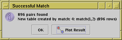
Pair plot completion confirmation dialogue
If you click the OK button, it will simply dismiss the dialogue. However, if you click the Plot Result button, a new plot window will appear with all the points from the input catalogues and pair links (lines between the joined positions) for the joined rows. The result is something like this:
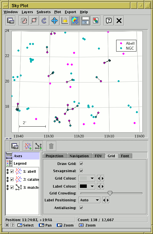
Output from crossmatch Plot Result
It shows clearly which points have been joined. You can fiddle with the plot controls in the usual way to adjust the output (see Appendix A.4). It is also possible to set up such plots by hand.
This section provides a bit more detail on the how the row matching of local tables (sections Section 5.2 and Section 5.3) is done. It is designed to give a rough idea to interested parties; it is not a tutorial description from first principles of how it all works.
The basic algorithm for matching is based on dividing up the space of possibly-matching rows into an (indeterminate) number of bins. These bins will typically correspond to disjoint cells of a physical or notional coordinate space, but need not do so. In the first step, each row of each table is assessed to determine which bins might contain matches to it - this will generally be the bin that it falls into and any "adjacent" bins within a distance corresponding to the matching tolerance. A reference to the row is associated with each such bin. In the second step, each bin is examined, and if two or more rows are associated with it every possible pair of rows in the associated set is assessed to see whether it does in fact constitute a matched pair. This will identify all and only those row pairs which are related according to the selected match criteria. During this process a number of optimisations may be applied depending on the details of the data and the requested match.
The matching algorithm described above is roughly an O(N log(N)) process, where N is the total number of rows in all the tables participating in a match. This is good news, since the naive interpretation would be O(N2). This can break down however if the matching tolerance is such that the number of rows associated with some or most bins gets large, in which case an O(M2) component can come to dominate, where M is the number of rows per bin. The average number of rows per bin is reported in the logging while a match is proceeding, so you can keep an eye on this.
For more detail on the matching algorithms, see the
javadocs for the uk.ac.starlink.table.join package,
or contact the author.
TOPCAT provides a number of facilities for positional crossmatches against tables which are exposed via Virtual Observatory web services (Cone Search, Simple Image Access and Simple Spectral Access) and general SQL-like matching (TAP). These work rather differently from the other functions described in this section, which operate on local tables, though conceptually the result is similar. See Section 6 for more details.
It also provides access to the X-Match service provided by the CDS, as described in Appendix A.11.1, which allows fast matching against any VizieR table or SIMBAD.
In many cases the CDS Upload X-Match window is the easiest, fastest and best way to match against remote tables. TAP is more flexible, but has a somewhat steeper learning curve, and may not be as fast or scalable for large local tables. The multi-SIA and multi-SSA windows may be useful for performing per-row searches of modest size against remote image or spectral archives. The multi-cone window is (since version 4.2) present mostly for historical reasons, and is not usually a good choice, since it is much less efficient than TAP or CDS X-Match.
Several of the windows in TOPCAT allow you to interface with so-called Data Access Layer services provided within the Virtual Observatory (VO). The buzzwords are not important, but the basic idea is that this allows you to locate a service providing data which may be of interest to you, and then query that service to obtain the data. The VO is not a single monolithic entity, but a set of protocols which allow a general purpose tool such as TOPCAT to talk to services made available by many different participating data providers in a uniform way, without having to have prior knowledge of what services are out there or the details of how their data is arranged.
The basic operation is similar for all of TOPCAT's access to these services:
These ideas are explained in more detail in the following subsections. The windows from which this is done are documented in Appendix A.9.
Note: For information on SAMP or PLASTIC, which are protocols developed within the Virtual Observatory context, but are not necessarily concerned with remote data access, see Section 9.
The Registry is fundamental to the way that the VO works. A registry is a list of all the services made available by different data providers. Each entry records some information about the type of service, who provided it, what kind of data it contains, and so on (registries may contain other types of entry as well, but we will not discuss these further here). Any data provider can add an entry to the registry to advertise that it has certain datasets available for access.
Several registries exist; they tend to be maintained by different regional VO organisations. At the time of writing, there are registries maintained for public access by GAVO, ESA, STScI and (remnants of) the UK's AstroGrid, amongst others. Particular projects may also maintain their own registries with limited holdings for internal use. The main public access registries talk to each other to synchronize their contents, so to a first approximation, they contain similar lists of entries to each other, and it shouldn't matter too much which one you use. In practice, there are some differences of format and content between them, so one may work better than another for you or may contain a record that you need. In most cases though, using the default registry (currently the GAVO one) will probably do what you want it to.
A number of different service types are defined and listed in the registry; the ones that TOPCAT currently knows how to access are the following:
Cone Search, SIA and SSA are positional protocols meaning that they query a single region of the sky. TOPCAT provides access to these service types in two main ways:
TAP is a much more powerful protocol not restricted to positional queries, and has its own interface. See the TAP load dialogue section in Appendix A.9.
Some services in the Virtual Observatory are authenticated, meaning that you have to log in to use them, or in some cases that you can optionally log in to gain additional rights, such as access to protected datasets or increased resource usage limits. Authentication for these situations mostly behaves as you would expect for an application working with external restricted services, but the details are given below.
If you attempt to access data which is restricted to authorised users, a window will pop up asking you to supply your username and password. Information about the URL you are trying to access will be displayed, so if you are authorized to use the service in question you will hopefully be able to supply the relevant login information. Additional information about how the authentication will be done may also be shown. If you log in successfully data access will proceed as expected, otherwise it will be blocked. Additionally, in the TAP Window you can log in to services for which authentication is optional by using the Log In/Out button.
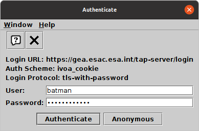
Authentication popup dialogue
Following a successful login attempt, subsequent access to similarly restricted data from the same source should make use of the same authentication information, so it ought not to be necessary to log in to the same service more than once, though in some cases the session might expire after some time, in which case a new login would be required.
If you find yourself logged in to services that you don't
want to be logged into any more (perhaps because you want to authenticate
as a different user),
you can log out of all currently authenticated services using
the Reset Authentication ( ) action
in the main control window File menu.
) action
in the main control window File menu.
Authentication status does not persist between TOPCAT sessions, so you will have to log in again to services every time you run the application.
Note: These authentication arrangements in TOPCAT are new at version 4.9, and rely on VO standards that are still under discussion. The behaviour and user interface may change in future releases, and at time of writing not all data services that provide authentication advertise it in a way that TOPCAT can work with. It is hoped that authentication interoperability will improve in future versions of TOPCAT and of server-side software.
TOPCAT allows you to enter algebraic expressions in a number of contexts:
What you write are actually expressions in the Java language, which are compiled into Java bytecode before evaluation. However, this does not mean that you need to be a Java programmer to write them. The syntax is pretty similar to C, but even if you've never programmed in C most simple things, and some complicated ones, are quite intuitive.
The following explanation gives some guidance and examples for writing these expressions. Unfortunately a complete tutorial on writing Java expressions is beyond the scope of this document, but it should provide enough information for even a novice to write useful expressions.
The expressions that you can write are basically any function of all the column values and subset inclusion flags which apply to a given row; the function result can then define the per-row value of a new column, or the inclusion flag for a new subset, or the action to be performed when a row is activated by clicking on it. If the built-in operators and functions are not sufficient, or it's unwieldy to express your function in one line of code, you can add new functions by writing your own classes - see Section 7.11.
Note: if Java is running in an environment with certain security restrictions (a security manager which does not permit creation of custom class loaders) then algebraic expressions won't work at all, and the buttons which allow you to enter them will be disabled.
To create a useful expression for a cell in a column, you will have to refer to other cells in different columns of the same table row. You can do this in three ways:
ucd$<ucd-spec>". Depending on the version of
UCD scheme used, UCDs can contain various punctuation marks such
as underscores, semicolons and dots; for the purpose of this syntax
these should all be represented as underscores ("_").
So to identify a column which has the UCD "phot.mag;em.opt.R",
you should use the identifier "ucd$phot_mag_em_opt_r".
Matching is not case-sensitive. Futhermore, a trailing underscore
acts as a wildcard, so that the above column could also be referenced
using the identifier "ucd$phot_mag_". If multiple
columns have UCDs which match the given identifer, the first one
will be used.
Note that the same syntax can be used for referencing table parameters (see Section 7.3); columns take preference so if a column and a parameter both match the requested UCD, the column value will be used.
utype$<utype-spec>".
Utypes can contain various punctuation marks such as colons and dots;
for the purpose of this syntax
these should all be represented as underscores ("_").
So to identify a column which has the Utype
"ssa:Access.Format",
you should use the identifier
"utype$ssa_Access_Format".
Matching is not case-sensitive.
If multiple columns have Utypes which match the given identifier,
the first one will be used.
Note that the same syntax can be used for referencing table parameters (see Section 7.3); columns take preference so if a column and a parameter both match the requested Utype, the column value will be used.
valueDouble, valueInt, valueLong,
valueString and valueObject
to obtain the typed value of a column with a given name.
The argument of the function is a string giving the exact
(case-sensitive) column name, for instance
valueDouble("b_E(BP-RP)")
will yield the value of the column named "b_E(BP-RP)"
as a double-precision floating point value.
These functions are not the generally recommended way
to get column values,
since they are slower and provide less type-checking than
the other options listed above,
and can occasionally lead to some other esoteric problems.
However, if you need to refer by name to strangely-named columns
they are sometimes a convenient option.
Object$"
before its identifier
(e.g. "Object$BMAG" for a column named BMAG)
the result will be the column value as a java Object.
Without that prefix, numeric columns are evaluated as java primitives.
In most cases, you don't want to do this,
since it means that you can't use the value in arithmetic expressions.
However, if you need the value to be passed to a
(possibly user-defined activation) method,
and you need that method to be invoked even when the value is null,
you have to do it like this. Null-valued primitives
otherwise cause expression evaluation to abort.
The value of the variables so referenced will be a primitive
(boolean, byte, short, char, int, long, float, double) if the
column contains one of the corresponding types. Otherwise it will
be an Object of the type held by the column, for instance a String.
In practice this means: you can write the name of a column, and it will
evaluate to the numeric (or string) value that that column contains
in each row. You can then use this in normal algebraic expressions
such as "B_MAG-U_MAG" as you'd expect.
If you have any Row Subsets defined you can also access the value of the boolean (true/false) flag indicating whether the current row is in each subset. Again there are two ways of doing this:
Note: in early versions of TOPCAT the hash sign ("#") was used instead of the underscore for this purpose; the hash sign no longer has this meaning.
? :" operator or
when combining existing subsets using logical operators to create
a new subset.
Some tables have constant values associated with them; these may represent such things as the epoch at which observations were taken, the name of the catalogue, an angular resolution associated with all observations, or any number of other things. Such constants are known as table parameters and can be viewed and modified in the Parameter Window. The values of such parameters can be referenced in algebraic expressions as follows:
param$.
ucd$. Any punctuation marks in the
UCD should be replaced by underscores, and a trailing underscore
is interpreted as a wildcard. See Section 7.1 for
more discussion.
utype$. Any punctuation marks in the
Utype should be replaced by underscores. See Section 7.1 for
more discussion.
As well as values defined by the tables you're working with, you can introduce independent variables into your expressions. At any given time these have a fixed value (they don't vary between rows of a table), but you can adjust them interactively using the Variables Window with a slider or by typing in a number. They are not attached to any single table.
This means you can for instance set up a parameterised expression for a synthetic column or subset, and then change the value of the parameter without having to edit the algebraic expression used for the column or subset definition.
By default, adjustments to these variables have an instant
effect on plots or other displays that depend on the values so defined.
That's usually what you want, but if very large or numerous plots
depend on a given variable, adjusting it can cause a lot of computation
or I/O and slow things down.
The plot windows therefore have a
Replot on Data Change ( ) button
that allow you to prevent such immediate updates, which will then
only take place on a replot which is triggered in some other way.
) button
that allow you to prevent such immediate updates, which will then
only take place on a replot which is triggered in some other way.
By default two global variables are set up and visible in the
Variables Window,
a floating point one var$x
and an integer one var$i,
and they are referenced in the expression language using these names.
But you can define new ones with names of your choice as well.
There are a few pseudo-variables which have special functions in the expression language. The following specials are column-like, in that they have a different value for each row:
$index or $0
long (8-byte integer);
when using it in certain expressions you may find it necessary to convert
it to an int (4-byte integer) using the
toInteger() function.
The deprecated alias "INDEX" may also be used.
$index0 or $00
$random (Deprecated)
0<=x<1.
NOTE: this token is deprecated since it can behave
unpredictably (the same cell does not always yield the same result).
Use instead the random() function in class
Maths.
The following specials are parameter-like, in that their value is not sensitive to the row:
$nrow
long (8-byte integer);
when using it in certain expressions you may find it necessary to convert
it to an int (4-byte integer) using the
toInteger() function.
$ncol
$nrow0
$nrow if a non-default
current subset is selected.
$ncol0
$ncol if some columns are
currently hidden.
When no special steps are taken, if a null value (blank cell) is encountered in evaluating an expression (usually because one of the columns it relies on has a null value in the row in question) then the result of the expression is also null.
It is possible to exercise more control than this, but it
requires a little bit of care,
because the expressions work in terms of primitive values
(numeric or boolean ones) which don't in general have a defined null
value. The name "null" in expressions gives you the java null
reference, but this cannot be matched against a primitive value
or used as the return value of a primitive expression.
For most purposes, the following two tips should enable you to work with null values:
NULL_"
(use upper case) to the column name or $ID. This
will yield a boolean value which is true if the column contains
a blank or a floating point NaN (not-a-number) value,
and false otherwise.
Note that if combined with other boolean expressions,
this null test should come first, i.e. write
"NULL_i || i==999" rather than
"i==999 || NULL_i",
though this is only essential for integer or boolean variables.
NULL"
(upper case). To return a null value from a non-numeric expression
(e.g. a String column) use the name "null" (lower case).
Null values are often used in conjunction with the conditional
operator, "? :"; the expression
test ? tval : fvalreturns the value
tval if the boolean expression test
evaluates true, or fval if test evaluates false.
So for instance the following expression:
Vmag == -99 ? NULL : Vmagcan be used to define a new column which has the same value as the Vmag column for most values, but if Vmag has the "magic" value -99 the new column will contain a blank. The opposite trick (substituting a blank value with a magic one) can be done like this:
NULL_Vmag ? -99 : VmagSome more examples are given in Section 7.10.
Note that for floating point data,
TOPCAT treats null and NaN (Not-a-Number) values
somewhat interchangeably.
Blank values arising either from an input file format that can represent
missing values, or from processing that fails to provide a definite value,
are in most cases represented internally as null
for integer-type values and NaN for floating point values.
However in general users should not rely on distinguishing between
null and NaN.
The operators are pretty much the same as in the C language. The common ones are:
+ (add)
- (subtract)
* (multiply)
/ (divide)
% (modulus)
! (not)
&& (and)
|| (or)
^ (exclusive-or)
== (numeric identity)
!= (numeric non-identity)
< (less than)
> (greater than)
<= (less than or equal)
>= (greater than or equal)
<, >, <=, >=,
== and !=
can be used on Strings as well as numeric values with common-sense meanings
(comparison based on Locale-specific string ordering);
this is a feature of the JEL-based expression language even though
it doesn't work like that in the Java language itself.
& (and)
| (or)
^ (exclusive-or)
<< (left shift)
>> (right shift)
>>> (logical right shift)
(byte) (numeric -> signed byte)
(short) (numeric -> 2-byte integer)
(int) (numeric -> 4-byte integer)
(long) (numeric -> 8-byte integer)
(float) (numeric -> 4-byte floating point)
(double) (numeric -> 8-byte floating point)
+ (string concatenation)
[] (array dereferencing - first element is zero)
?: (conditional switch)
instanceof (class membership)
Many functions are available for use within your expressions, covering standard mathematical and trigonometric functions, arithmetic utility functions, type conversions, and some more specialised astronomical ones. You can use them in just the way you'd expect, by using the function name (unlike column names, this is case-sensitive) followed by comma-separated arguments in brackets, so
max(IMAG,JMAG)
will give you the larger of the values in the columns IMAG and JMAG,
and so on.
The functions are grouped into the following classes:
Full documentation of the functions in these classes is given in Appendix B.1, and is also available within TOPCAT from the Available Functions Window.
This note provides a bit more detail for Java programmers on what is going on here; only read on if you want to understand how the use of functions in TOPCAT algebraic expressions relates to normal Java code.
The expressions which you write are compiled to Java bytecode
when you enter them (if there is a 'compilation error' it will be
reported straight away). The functions listed in the previous subsections
are all the public static methods of the classes which
are made available by default. The classes listed are all in the
packages uk.ac.starlink.ttools.func and
uk.ac.starlink.topcat.func
(uk.ac.starlink.topcat.func.Strings etc).
However, the public static methods are all imported into an anonymous
namespace for bytecode compilation, so that you write
sqrt(x) and not Maths.sqrt(x).
The same happens to other classes that are imported (which can be
in any package or none) - their public
static methods all go into the anonymous namespace. Thus, method
name clashes are a possibility.
This cleverness is all made possible by the rather wonderful JEL.
There is another category of functions which can be used apart from those listed in the previous section. These are called, in Java/object-oriented parlance, "instance methods" and represent functions that can be executed on an object.
It is possible to invoke any of its public
instance methods on any object
(though not on primitive values - numeric and boolean ones).
The syntax is that you place a "." followed by the method invocation
after the object you want to invoke the method on,
hence NAME.substring(3) instead of substring(NAME,3).
If you know what you're doing, feel free to go ahead and do this.
However, most of the instance methods you're likely to want to use
have equivalents in the normal functions listed in the previous section,
so unless you're a Java programmer or feeling adventurous, you are
probably best off ignoring this feature.
Here are some general examples. They could be used to define synthetic columns or (where numeric) to define values for one of the axes in a plot.
(first + second) * 0.5
sqrt(variance)
    radiansToDegrees(DEC_radians)
    degreesToRadians(RA_degrees)
    parseInt($12)
    parseDouble(ident)
toString(index)
     toShort(obs_type)
     toDouble(range)
or
    (short) obs_type
    (double) range
    hmsToDegrees(RA1950)
    dmsToDegrees(decDeg,decMin,decSec)
    degreesToDms($3)
    degreesToHms(RA,2)
min(1000, max(value, 0))
jmag == 9999 ? NULL : jmag
NULL_jmag ? 9999 : jmag
psfCounts[2]
"MLT".indexOf(spType.charAt(0)) * 10 + parseDouble(substring(spType,1)) + 10Note this uses a couple of Java String instance methods (Section 7.9) which are not explicitly documented in this section.
RA > 100 && RA < 120 && Dec > 75 && Dec < 85
    $2*$2 + $3*$3 < 1
    skyDistanceDegrees(ra0,dec0,hmsToDegrees(RA),dmsToDegrees(DEC))<15./3600.
index <= 100
index % 10 == 0
    equals(SECTOR, "ZZ9 Plural Z Alpha")
    equalsIgnoreCase(SECTOR, "zz9 plural z alpha")
    startsWith(SECTOR, "ZZ")
    contains(ph_qual, "U")
matches(SECTOR, "[XYZ] Alpha")
_1 && _2
_1 || _2
(in_cluster && has_photometry) || ! _6
! NULL_ellipticity
The functions provided by default for use with algebraic expressions, while powerful, may not provide all the operations you need. For this reason, it is possible to write your own extensions to the expression language. In this way you can specify arbitrarily complicated functions. Note however that this will only allow you to define new columns or subsets where each cell is a function only of the other cells in the same row - there is no way to define a value in one row as a function of values in other rows.
In order to do this, you have to write and compile a (probably short) program in the Java language. A full discussion of how to go about this is beyond the scope of this document, so if you are new to Java and/or programming you may need to find a friendly local programmer to assist (or mail the author). The following explanation is aimed at Java programmers, but may not be incomprehensible to non-specialists.
The steps you need to follow are:
jel.classes or jel.classes.activation
system properties (colon-separated if there are several)
as described in Section 10.2.3
or during a run using the
Available Function Window's
Add Class () buttonAny public static methods defined in the classes thus specified will be available for use in the Synthetic Column, Algebraic Subset or (in the case of activation functions only) Activation windows. They should be defined to take and return the relevant primitive or Object types for the function required (in the case of activation functions the return value should normally be a short log string).
For example, a class written as follows would define a three-value average:
    public class AuxFuncs {
        public static double average3(double x, double y, double z) {
            return (x + y + z) / 3.0;
        }
    }
and the expression
"average3($1,$2,$3)"
could then be used to define a new synthetic column, giving the average of
the first three existing columns.
Exactly how you would build this is dependent on your system,
but it might involve doing something like the following:
javac AuxFuncs.java"topcat -Djel.classes=AuxFuncs -classpath ."Note that (in versions later than TOPCAT 4.3-2) variable-length argument lists are supported where the final declared argument is an array, so for instance a method declared like:
       public static double sum(double[] values) {
           double total = 0;
           for (int i = 0; i < values.length; i++) {
               total += values[i];
           }
           return total;
       }
can be invoked like "sum(UMAG,GMAG,RMAG,IMAG,ZMAG)".
The alternative form "double... values" can be used in
the declaration with identical effect.
Note that the activation action framework has changed considerably at TOPCAT v4.6. It is now much more flexible than in previous versions.
As well as seeing the overview of table data provided by a plot or statistics summary, it is often necessary to focus on a particular row of the table, which according to the nature of the table may represent an astronomical object, an event or some other entity. In the Data Window a table row is simply a row of the displayed JTable, and in a scatter plot it corresponds to one plotted point.
If you click on a plotted point in one of the graphics windows, or on a row in the Data Window (or in a few other circumstances - see below) the corresponding table row will be activated. When a row is activated, four things happen:
The fourth item is much more flexible. By using the Activation Window, you can set up one or several configurable events to take place on row activation. Examples include things like viewing a cutout image near the activated row's sky position or sending the sky position to an external all-sky viewer so that it displays that region of the sky. So for instance having spotted an interesting point in a plot of a galaxy catalogue you can click on it, and immediately see an observed image to identify its morphological type. Other options include communicating with external applications using SAMP for each activated row, for instance asking an image viewer such as DS9 to load an image in a table ImageURL column. All the options, along with details of how to configure them, are listed in Appendix A.10.1. Since v4.6-1, all the defined Activation Actions are saved when you save the session (though not if you just save the table).
If none of these options fits your particular requirements,
there are various ways to implement custom behaviour.
One is to invoke some kind of external program such as a
shell script, and pass parameters to it based on row values;
this can be done using the
Run system command option.
You can also execute custom code in TOPCAT's
expression language
using the Execute code option
using some activation functions
specially provided to perform useful actions
(e.g. image display) rather than just return results.
Finally, advanced users can supply their own activation functions
for use with the Execute Code option,
or can implement their own activation actions
and plug them in at runtime using the topcat.activators
system property.
A row can be activated in the following circumstances:
table.highlight.row
SAMP messageTOPCAT is able to communicate with other tools using one or other of two messaging protocols:
An example of the kind of thing which can be done might be:SAMP and PLASTIC do much the same job as each other, and work in much the same way. SAMP is an evolution of PLASTIC with a number of technical improvements, and PLASTIC has been deprecated in favour of SAMP since around 2009. PLASTIC is therefore of mainly historical interest, though TOPCAT can still run in PLASTIC mode on request, if you need it to communicate with older tools that can only speak PLASTIC.
The communication architecture of the two protocols is basically the same: all tools communicate with a central "Hub" process, so a hub must be running in order for the messaging to operate. If a hub is running when TOPCAT starts, or if one starts up while TOPCAT is in operation, it will connect to it automatically. If no SAMP hub is running, TOPCAT will set one up during application startup.
TOPCAT can work in either SAMP or PLASTIC mode, but not both at once.
It determines which mode to use at startup:
if the -samp or -plastic flag is supplied
on the command line the corresponding mode will be used;
otherwise it will try to use SAMP.
It is easy to tell which mode is being used by looking at the
Control Window;
in SAMP mode the SAMP panel displaying connection
and message status is visible at the bottom of the right hand panel
(there are a few other changes to the GUI as well).
This communication has two aspects to it: on the one hand TOPCAT can send messages to other applications which causes them to do things, and on the other hand TOPCAT can receive and act on such messages sent by other applications. The sent and received messages are described separately in the subsections below. There are also sections on the, somewhat different, ways to control and monitor messaging operatiion for the cases of SAMP and PLASTIC.
Note that the new activation action framework introduced in TOPCAT v4.6, unlike the activation window in previous versions, in most cases only works with SAMP and not PLASTIC.
When running in SAMP mode, the Control Window features several ways to view and control SAMP status.
 )
) and Table Send (
)
) and Table Send ( )
menu options
)
menu options
 ) menu option
A number of other windows feature an Interop menu with
Broadcast () and
Send ()
operations for data types appropriate to that window.
Sometimes Broadcast appears in the toolbar as well.
In some cases there are also Accept ( )
toggle options in the Interop menu.
These control whether TOPCAT will respond to appropriate messages sent
by other SAMP applications.
)
toggle options in the Interop menu.
These control whether TOPCAT will respond to appropriate messages sent
by other SAMP applications.
Note: the PLASTIC protocol has been deprecated in favour of SAMP since about 2009, and this functionality, though still present, is of mostly historical interest.
You can view and control operations relating to the PLASTIC hub from the Interop menu in the Control Window. It contains the following options:
kill command).
Because this has some system-dependent features, it's not guaranteed to
work, especially in non-Unix environments.
Help on interoperability
Broadcast Table
Send Table to ...
This section describes the messages which TOPCAT can transmit to other tools which understand the SAMP or PLASTIC protocol, and how to cause them to be sent. Approximately the same behaviour results for either SAMP or PLASTIC, except as noted.
In most cases you can choose two ways to transmit a message from TOPCAT:
Broadcast
Send
Below is a list of places you can cause TOPCAT to transmit messages. The SAMP MTypes and PLASTIC message IDs are listed along with the descriptions; unless you are a tool developer you can probably ignore these.
The Send VOTable activation action also sends this message (SAMP only).
SAMP MTypes:
table.load.votable or
table.load.fits
PLASTIC Message IDs:
ivo://votech.org/votable/load or
ivo://votech.org/votable/loadFromURL
Also, whenever a new subset is created, for instance by entering an algebraic expression or tracing out a region on a plot (see Section 3.1.1), you have the option of transmitting the subset directly to one or all listening applications as an alternative to adding the new subset to the table's subset list.
SAMP MType: table.select.rowList
PLASTIC Message ID: ivo://votech.org/votable/showObjects
SAMP MType: table.highlight.row
SAMP MType: coord.pointAt.sky
The (old-style, somewhat deprecated) Density Plot window also produces a 2-d histogram which is actually an image, and this can be sent to image applications from its Interop menu.
SAMP MType: image.load.fits
PLASTIC Message ID: ivo://votech.org/fits/image/loadFromURL
SAMP MType: spectrum.load.ssa-generic
SAMP MTypes: voresource.loadlist.cone,
voresource.loadlist.siap,
voresource.loadlist.ssap
This section describes the messages which TOPCAT will respond to when it receives them from other applications via the SAMP/PLASTIC hub. The SAMP MTypes and PLASTIC message IDs are listed along with the descriptions; unless you are a tool developer you can probably ignore these.
SAMP MType:
table.load.votable,
table.load.fits,
table.load.cdf,
table.load.pds4,
table.load.stil or
coverage.load.moc.fits.
PLASTIC Message ID:
ivo://votech.org/votable/load or
ivo://votech.org/votable/loadFromURL
Note the non-standard MType table.load.stil is
supported for loading tables with SAMP. This is like the other
table.load.* MTypes, but any table format supported
by the application is permitted. This MType has an additional
parameter "format", which must contain the table format
name (not case sensitive).
Note: this behaviour differs from the behaviour in TOPCAT versions prior to v3.0. Different options for handling exactly how a received row selection is treated may be made available in future versions.
SAMP MType: table.select.rowList
PLASTIC Message ID: ivo://votech.org/votable/showObjects
SAMP MType: table.highlight.row
PLASTIC Message ID: ivo://votech.org/votable/highlightObject
SAMP MTypes: voresource.loadlist,
voresource.loadlist.cone,
voresource.loadlist.siap,
voresource.loadlist.ssap
format
giving the (case-insensitive) table format name required for
the output table.
It also takes an optional integer-like parameter id,
giving the ID number (as shown in the Control Window table list)
of the table required. If id is missing or non-positive,
the current table is used.
The returned response has an output parameter url
giving the URL of the apparent table in question.
This MType is experimental and may be modified or withdrawn in
the future.
SAMP MType: table.get.stil.
System-level messages are also responded to. For SAMP these are:
samp.hub.disconnect
samp.hub.event.shutdown
samp.hub.event.register
samp.hub.event.unregister
samp.hub.event.metadata
samp.hub.event.subscriptions
samp.app.ping
ivo://votech.org/test/echo
ivo://votech.org/info/getName
ivo://votech.org/info/getIconURL
ivo://votech.org/hub/event/ApplicationRegistered
ivo://votech.org/hub/event/ApplicationUnregistered
ivo://votech.org/hub/event/HubStopping
Starting up TOPCAT may just be a case of typing "topcat" or
clicking on an appropriate icon and watching the
Control Window pop up.
If that is the case, and it's running happily for you,
you can probably ignore this section.
What follows is a description of how to start the program up,
and various command line arguments and configuration options which can't be
changed from within the program.
Some examples are given in Section 10.5.
Actually obtaining the program is not covered here; please see
the TOPCAT web page
http://www.starlink.ac.uk/topcat/.
There are various ways of starting up TOPCAT depending on how (and whether) it has been installed on your system; some of these are described below.
There may be some sort of short-cut icon on your desktop which
starts up the program - in this case just clicking on it will probably work.
Failing that you may be able to locate the
jar file (probably named topcat.jar,
topcat-full.jar or
topcat-extra.jar)
and click on that. These files would be located in the
java/lib/topcat/ directory in a standard Starjava installation.
Note that when you start by clicking on something
you may not have the option of entering
any of the command line options described below -
to use these options, which you may need to do for serious use of
the program, you will have to run the program from the command line.
Alternatively you will have to invoke the program from the command line.
On Unix-like operating systems, you can use the topcat script.
If you have the full starjava installation, this is probably in
the starjava/java/bin directory. If you have one of the
standalone jar files (topcat-*.jar), it should
be in the same directory as it/them. If it's not there,
you can unpack it from the jar file itself, using a command like
unzip topcat-full.jar topcat.
If that directory (and java) is on your path then you can write:
topcat [java-args] [topcat-args]In this case any arguments which start
-D or -X
are assumed to be arguments to the java command,
any arguments which start -J are stripped of the -J
and then passed as arguments to the java command,
a -classpath path defines a class path to
be used in addition to the TOPCAT classes,
and any remaining arguments are used by TOPCAT.
If you're not running Unix then to start from the
command line you will have to use the java command itself.
The most straightforward way of doing this will look like:
java [java-args] -jar path/to/topcat.jar [topcat-args](or the same for
topcat-full.jar etc).
However NOTE: using java's -jar flag ignores
any other class path information, such as the CLASSPATH environment
variable or java's -classpath flag - see Section 10.2.1.
The meaning of the optional
[topcat-args]
and
[java-args]
sequences are described in
Section 10.1 and
Section 10.2 below respectively.
You can start TOPCAT from the command line with no arguments - in this case it will just pop up the command window from which you can load in tables. However you may specify flags and/or table locations and formats.
If you invoke the program with the "-help" flag you
will see the following usage message:
Usage: topcat <flags> [[-f <format>] <table> ...]

    General flags:
        -help          print this message and exit
        -version       print component versions etc and exit
        -verbose       increase verbosity of reports to console
        -debug         add debugging information to console log messages
        -demo          start with demo data
        -running       use existing TOPCAT instance if one is running
        -memory        use memory storage for tables
        -disk          use disk backing store for large tables
        -samp          use SAMP for tool interoperability
        -plastic       use PLASTIC for tool interoperability
        -[no]hub       [don't] run internal SAMP/PLASTIC hub
        -exthub        run external SAMP/PLASTIC hub
        -noserv        don't run any services (PLASTIC or SAMP)
        -nocheckvers   don't check latest version
        -stilts <args> run STILTS not TOPCAT
        -jsamp <args>  run JSAMP not TOPCAT

    Useful Java flags:
        -classpath jar1:jar2..  specify additional classes
        -XmxnnnM                use nnn megabytes of memory
        -Dname=value            set system property

    Auto-detected formats:
        fits-plus, colfits-plus, colfits-basic, fits, votable, cdf, ecsv, pds4, mrt, parquet, feather, gbin

    All known formats:
        fits-plus, colfits-plus, colfits-basic, fits, votable, cdf, ecsv, pds4, mrt, parquet, feather, gbin, ascii, csv, tst, ipac, hapi, ver, wdc

    Useful system properties (-Dname=value - lists are colon-separated):
        java.io.tmpdir          temporary filespace directory
        jdbc.drivers            JDBC driver classes
        jel.classes             custom algebraic function classes
        jel.classes.activation  custom action function classes
        star.connectors         custom remote filestore classes
        startable.load.dialogs  custom load dialogue classes
        startable.readers       custom table input handlers
        startable.writers       custom table output handlers
        startable.storage       storage policy
        mark.workaround         work around mark/reset bug
            (see topcat -jsamp -help for more)
The meaning of the flags is as follows:
-f flag what format the named files are in.
Any table file on the command line following a
-f <format>
sequence must be in the named format until the next -f flag.
The names of both the auto-detected formats (ones which don't need
a -f) and the non-auto-detected formats (ones which do)
are given in the usage message you can see by giving the
-help flag (this message is shown above).
You may also use the classname of a class on the classpath which
implements the TableBuilder interface -
see SUN/252.
-help (or -h)
flag is given, TOPCAT will write a usage
message and exit straight away.
-version flag is given, TOPCAT will print
a summary of its version and the versions and availability of some
its components, and exit straight away.
-verbose (or -v) flag increases
the level of verbosity of messages which TOPCAT writes to standard
output (the console).
It may be repeated to increase the verbosity further.
The messages it controls are currently those written through
java's standard logging system - see the description of the
Log Window for more
information about this.
-debug flag affects how logging messages appear
(whether they appear is affected by the -verbose flag).
If present, these messages will provide more detail about where
each message was generated from.
-demo flag causes the program to start up with
a few demonstration tables loaded in. You can use these to play
around with its facilities. Note these demo tables are quite small
to avoid taking up a lot of space in the installation, and don't
contain particularly sensible data, they are just to give an idea.
-running flag can be used when specifying tables
on the command line. If an existing instance of TOPCAT is already
running, the tables are loaded into it. If no instance of TOPCAT
is running (or at least one cannot be discovered), then the
-running flag has no effect and a new instance is
started up as usual.
-memory flag is given then the program will
store table data in memory,
rather than the default which is to store small tables in memory,
and larger ones in temporary disk files.
-disk flag is given then the program will
store table data in temporary disk files,
rather than the default which is to store small tables in memory,
and larger ones on disk.
If you get out of memory messages, running with the -disk
flag might help, though the default policy should work fairly well.
The temporary data files are written in the default temporary
directory (defined by the java.io.tmpdir system property -
often /tmp - and deleted when the program exits, unless
it exits in an unusual way.
-hub flag causes TOPCAT to run an internal
SAMP or PLASTIC hub (SAMP by default), if no hub is already
running, and the -nohub flag prevents this from happening.
The default behaviour, when neither of these flags is given,
is to start a hub automatically for
SAMP but not for PLASTIC. The hub will terminate when TOPCAT does,
or can be shut down manually with the
Interop|Stop Internal Hub () menu item.
See Section 9.
topcat -stilts -help)
for the form of the <stilts-args>.
topcat -jsamp -help
for more information.
Other arguments on the command line are taken to be the locations of tables. Any tables so specified will be loaded into TOPCAT at startup. These locations are typically filenames, but could also be URLs or scheme specifications. In addition they may contain "fragment identifiers" (with a "#") to locate a table within a given resource, so that for instance the location
/my/data/cat1.fits#2means the second extension in the multi-extension FITS file
/my/data/cat1.fits.
Section 4.2 describes in more detail the
kinds of URLs which can be used here.
Note that options to Java itself may also be specified on the command-line, as described in the next section.
As described above, depending on how you invoke TOPCAT you may be able to specify arguments to Java itself (the "Java Virtual Machine") which affect how it runs. These may be defined on the command line or in some other way. The following subsections describe how to control Java in ways which may be relevant to TOPCAT; they are however somewhat dependent on the environment you are running in, so you may experience OS-dependent variations.
The classpath is the list of places that Java looks to find the bits of compiled code that it uses to run an application. When running TOPCAT this always has to include the TOPCAT classes themselves - this is part of the usual invocation and is described in Section 10. However, for certain things Java might need to find some other classes, in particular for:
If you are going to use these facilities you will need to start the
program with additional class path elements that point to the location
of the classes required. How you do this depends on how you
are invoking TOPCAT.
If you are using tht topcat startup script, you can write:
topcat -classpath other-paths ...
(this adds the given paths to the standard ones required for TOPCAT itself).
If you are invoking java directly, then you can either write on the
command line:
    java -classpath path/to/topcat.jar:other-paths
         uk.ac.starlink.topcat.Driver ...
or set the CLASSPATH environment variable something like this:
setenv CLASSPATH path/to/topcat.jar:other-paths
In any case, multiple (extra) paths should be separated by colons
in the other-paths string.
Note that if you are running TOPCAT
using java's -jar flag,
any attempt you make to specify the classpath will be ignored!
This is to do with Java's security model.
If you need to specify a classpath which includes more than the
TOPCAT classes themselves, you can't use java -jar
(use
java -classpath topcat-full.jar:... uk.ac.starlink.topcat.Driver
instead).
If TOPCAT fails during operation with a message that says something
about a java.lang.OutOfMemoryError, then your heap
size is too small for what you are trying to do. You will have to
run java with a bigger heap size using the -Xmx flag.
Invoking TOPCAT from the topcat script you would write
something like:
topcat -Xmx256M ...
or using java directly:
java -Xmx256M ...
which means use up to 256 megabytes of memory (don't forget the "M"
for megabyte). JVMs often default to a heap size of 64M.
You probably don't want to specify a heap size larger than the
physical memory of the machine that you are running on.
There are other types of memory and tuning options controlled
using options of the form -X<something-or-other>;
if you're feeling adventurous you may be able to find out about these
by typing "java -X".
System properties are a way of getting information into Java (they are the Java equivalent of environment variables). The following ones have special significance within TOPCAT:
apple.laf.useScreenMenuBar
true for TOPCAT,
so menus mostly appear at the top of the screen (though it's not
true to say that TOPCAT obeys the Mac look and feel completely);
if you prefer the more Java-like look and feel, set it to
false.
http.proxyHost
http.proxyPort,
https.proxyHost etc.
See the appropriate java documentation
(e.g. by googling for "http.proxyHost") for details.
java.io.tmpdir
/tmp on Unix),
so if working with large unmapped (e.g. CSV) tables
on a machine with limited space on the default disk,
it may be necessary to change it.
java.util.concurrent.ForkJoinPool.common.parallelism
jdbc.drivers
jel.classes
jel.classes.activation
jsamp.hub.profiles
-hub/-exthub flag or
from the GUI).
The value is a comma-separated list of profile specifiers;
options are
"std" for Standard Profile,
"web" for Web Profile or
the name of a class implementing the
org.astrogrid.samp.hub.HubProfile interface.
The default setting runs just a Standard Profile hub,
but, for instance, setting it to "std,web" would run a
Web Profile as well. Note you should include std in
the list, otherwise TOPCAT will not be able to talk to the hub.
See the JSAMP documentation for more detail.
jsamp.localhost
127.0.0.1".
However, if this property is set (presumably to the local host's
fully- or partly-qualified domain name) its value will be used instead.
Two special values may also be set:
"[hostname]" for the host's fully qualified domain name, and
"[hostnumber]" for the IP number.
jsamp.server.port
jsamp.xmlrpc.impl
xml-log" or "rpc-log"
then all XML-RPC communications will be logged in very or fairly
verbose terms respectively to standard output.
The classname of an org.astrogrid.samp.xmlrpc.XmlRpcKit
implementation may be given instead to use a custom implementation.
lut.files
       1.0  1.0  0.0
       1.0  0.0  1.0
would give a colour map that fades from yellow to magenta. Any number of
samples may be given; the scale is interpolated.
mark.workaround
mark()/reset() methods of some java
InputStream classes. These are rather common,
including in Sun's J2SE system libraries.
Use this if you are seeing errors that say something like
"Resetting to invalid mark".
Currently defaults to "false".myspace.cache
service.maxparallel
auth.schemes
uk.ac.starlink.auth.AuthScheme implementation
classnames may be provided.
star.connectors
uk.ac.starlink.connect.Connector interface which
specifies how you can log on to such a service and provides a
hierarchical view of the filespace it contains.
startable.load.dialogs
uk.ac.starlink.table.gui.TableLoadDialog interface and
naming them in this property.
See STIL
documentation for more detail.
startable.readers
startable.schemes
uk.ac.starlink.table.TableScheme interface,
and must have a no-arg constructor.
The schemes thus named will be available
alongside the standard ones listed in Section 4.3.
startable.storage
disk" has basically the same effect as
supplying the "-disk" argument on the TOPCAT command line
(see Section 10.1).
Other possible values are "adaptive", "memory",
"sideways" and "discard";
see SUN/252.
The default is "adaptive", which means storing smaller
tables in memory, and larger ones on disk.
startable.unmap
sun" (the default),
"cleaner", "unsafe" or "none".
In most cases you are advised to leave this alone, but in the event of
unmapping-related JVM crashes (not expected!), setting it to
none may help.
startable.writers
topcat.activators
uk.ac.starlink.topcat.activate.ActivationType interface,
and which has a no-arg constructor.
topcat.exttools
uk.ac.starlink.topcat.TopcatToolAction interface and have a
no-arg constructor.
The actions corresponding to any such classes will be added to toolbar.
This is an experimental extensibility feature, which may be modified or
withdrawn in a future release.
user.dir
votable.namespacing
none" (no namespacing, xmlns declarations
in VOTable document will probably confuse parser),
"lax" (anything that looks like it is probably a VOTable
element will be treated as a VOTable element) and
"strict" (VOTable elements must be properly declared in one
of the correct VOTable namespaces).
May also be set to the classname of a
uk.ac.starlink.votable.Namespacing implementation.
The default is "lax".
votable.strict
FIELD or PARAM element with
a datatype attribute of
char/unicodeChar,
and no arraysize attribute.
The VOTable standard says this indicates a single character,
but some VOTables omit arraysize specification by accident when
they intend arraysize="*".
If votable.strict is set true,
a missing arraysize will be interpreted as meaning a single character,
and if false, it will be interpreted as a variable-length
array of characters (a string).
The default is true.
votable.version
1.0", "1.1",
"1.2", "1.3" or "1.4".
By default, version 1.4 VOTables are written.
To define these properties on the command line
you use the -D flag, which has the form
-D<property-name>=<value>
If you're using the TOPCAT startup script, you can write something like:
topcat -Djdbc.drivers=org.postgresql.Driver ...
or if you're using the java command directly:
java -Djdbc.drivers=org.postgresql.Driver ...
Alternatively you may find it more convenient to
write these definitions in a file named
.starjava.properties in your home directory; the above
command-line flag would be equivalent to inserting the line:
jdbc.drivers=org.postgresql.Driver
in your .starjava.properties file.
This section describes additional configuration which must be done to allow TOPCAT to access SQL-compatible relational databases for reading (see Appendix A.6.4) or writing (see Appendix A.7.2.4) tables. If you don't need to talk to SQL-type databases, you can ignore the rest of this section. The steps described here are the standard ones for configuring JDBC (which sort-of stands for Java Database Connectivity); you can find more information on that on the web. The best place to look may be within the documentation of the RDBMS you are using.
To use TOPCAT with SQL-compatible databases you must:
jdbc.drivers system property to the name of the
driver class as described in Section 10.2.3
Below are presented the results of some experiments with JDBC drivers. Note however that this information may be be incomplete and out of date. If you have updates, feel free to pass them on and they may be incorporated here.
To the author's knowledge, TOPCAT has so far successfully been used with the following RDBMSs and corresponding JDBC drivers:
useUnicode=true&characterEncoding=UTF8" may be required
to handle some non-ASCII characters.
jdbc:oracle:thin:@//hostname:1521/database#SELECT ...
for querying an existing database (loading) and
jdbc:oracle:thin:@//hostname:1521/database#new-table-name
for writing a new table (saving).
jdbc:sybase:Tds:hostname:port/dbname?user=XXX&password=XXX#SELECT...".
An earlier attempt using Sybase ASE 11.9.2 failed.
Here are some example command lines to start up TOPCAT using databases that at least have worked at some point.
   java -classpath topcat-full.jar:pg73jdbc3.jar \
        -Djdbc.drivers=org.postgresql.Driver \
        uk.ac.starlink.topcat.Driver
   java -classpath topcat-full.jar:mysql-connector-java-3.0.8-bin.jar \
        -Djdbc.drivers=com.mysql.jdbc.Driver \
        uk.ac.starlink.topcat.Driver
   java -classpath topcat-full.jar:ojdbc14.jar \
        -Djdbc.drivers=oracle.jdbc.driver.OracleDriver \
        uk.ac.starlink.topcat.Driver
   java -classpath topcat-full.jar:jtds-1.1.jar \
        -Djdbc.drivers=net.sourceforge.jtds.jdbc.Driver \
        uk.ac.starlink.topcat.Driver
Considerable effort has gone into making TOPCAT capable of dealing with large datasets. In particular it does not in general have to read entire files into memory in order to do its work, so it's not restricted to using files which fit into the java virtual machine's 'heap memory' or into the physical memory of the machine. As a rule of thumb, the program will work at reasonable speed with tables up to about 1-10 million rows, depending on the machine it's running on. It may well work work with hundreds of millions of rows, but performance may be more sluggish. The number of columns is less of an issue, though see below concerning performance.
However, the way you invoke the program affects how well it can cope with large tables; you may in some circumstances get a message that TOPCAT has run out of memory (either a popup or a terse "OutOfMemoryError" report on the console), and there are some things you can do about this:
-Xmx flag, followed by the maximum heap memory,
for instance "topcat -Xmx1000M" or
"java -Xmx1000M -jar topcat-full.jar".
Don't forget the "M" to indicate megabytes
or "G" for gigabytes.
It's generally reasonable to increase this value up to nearly the
amount of free physical memory in your machine if you need to
(taking account of the needs of other processes running at the same time)
but attempting any more will usually result in abysmal performance.
See Section 10.2.2.
-Xmx flags as above.
Feather format also has the same advantages.
java -version" (or "topcat -version")
will probably say something about 64-bit-ness if it is 64-bit.
It is also possible to use column-oriented storage for non-FITS
files by specifying the flag -Dstartable.storage=sideways.
This is like using the -disk flag but uses column-oriented
rather than row-oriented temporary files. However, using it for
such large files means that the conversion is likely to be rather
slow, so you may be better off converting the original file to
colfits format in a separate step and using that.
adaptive", means that the data for relatively small
tables are stored in memory, and for larger ones in temporary disk files.
This usually works fairly well and you're not likely to need to change it.
However, you can experiment if you like, and a small amount of
memory may be saved if you encourage it to store all table data on disk,
by specifying the -disk flag on the command line.
You can achieve the same effect by adding the line
startable.storage=disk in the
.starjava.properties in your home directory.
See Section 10.1, Section 10.2.3.
As far as performance goes, the memory size of the machine you're using does make a difference. If the size of the dataset you're dealing with (this is the size of the FITS HDU if it's in FITS format but may be greater or less than the file size for other formats) will fit into unused physical memory then general everything will run very quickly because the operating system can cache the data in memory; if it's larger than physical memory then the data has to keep being re-read from disk and most operations will be much slower, though use of column-oriented storage can help a lot in that case.
Here are some examples of invoking TOPCAT from the command line.
In each case two forms are shown: one using the topcat
script, and one using the jar file directly. In the latter case,
the java command is assumed to be on the your path, and
the jar file itself, assumed in directory my/tcdir,
might be named topcat.jar,
topcat-full.jar, or something else, but the form
of the command is the same.
    topcat
    java -jar topcat.jar
    topcat -h
    java -jar topcat.jar -h
    topcat testcat.fits
    java -jar my/tcdir/topcat.jar testcat.fits
    topcat t1.fits -f ascii t2.txt t3.txt -f votable t4.xml
    java -jar my/tcdir/topcat.jar t1.fits -f ascii t2.txt t3.txt -f votable t4.xml
    topcat -Xmx256M -disk
    java -Xmx256M -jar my/tcdir/topcat.jar -disk
    topcat -classpath my/funcdir/funcs.jar -Djel.classes=my.ExtraFuncs t1.fits
    java -classpath my/tcdir/topcat.jar:my/funcdir/funcs.jar \
         -Djel.classes=func.ExtraFuncs \
         uk.ac.starlink.topcat.Driver t1.fits
    topcat -classpath my/jdbcdir/pg73jdbc3.jar -Djdbc.drivers=org.postgresql.Driver
    java -classpath my/tcdir/topcat.jar:my/jdbcdir/pg73jdbc3.jar \
         -Djdbc.drivers=org.postgresql.Driver uk.ac.starlink.topcat.Driver
    topcat -classpath my/driverdir/drivers.jar \
           -Dstartable.readers=my.MyTableBuilder \
           -Dstartable.writers=my.MyTableWriter \
    java -classpath my/tcdir/topcat.jar:my/driverdir/drivers.jar \
         -Dstartable.readers=my.MyTableBuilder \
         -Dstartable.writers=my.MyTableWriter \
         uk.ac.starlink.topcat.Driver
-Dx=y definitions can be avoided by putting equivalent
x=y lines into the .starjava.properties in your
home directory.
This appendix gives a tour of all the windows that form the TOPCAT application, explaining the anatomy of the windows and the various tools, menus and other controls. Attributes common to many or all windows are described in Appendix A.1, and the subsequent sections describe each of the windows individually.
When the application is running, the Help For Window
() toolbar button will display the appropriate description
for the window on which it is invoked.
This section describes some features which are common to many or all of the windows used in the TOPCAT program.
Each window has a toolbar at the top containing various buttons representing actions that can be invoked from the window. Most of them contain the following buttons:
 Close
Help
Close
Help
Buttons in the toolbar often appear in menus of the same window as well; you can identify them because they have the same icon. This is a convenience; invoking the action from the toolbar or from the menu will have the same effect.
Often an action will only be possible in certain circumstances, for instance if some rows in the associated JTable have been selected. If the action is not possible (i.e. it would make no sense to invoke it) then the button in the toolbar and the menu option will be greyed out, indicating that it cannot be invoked in the current state.
Most windows have a menu bar at the top containing one or more menus. These menus will usually provide the actions available from the toolbar (identifiable because they have the same icons), and may provide some other less-commonly-required actions too.
Here are some of the menus common to several windows:
 Control Window
 Scrollable
Close
Exit
Scrollable
Close
Exit
 Help
Help for Window
Help
Help for Window
 Help in Browser
 Help in Browser (single page)
 Help for Window in Browser
 About TOPCAT
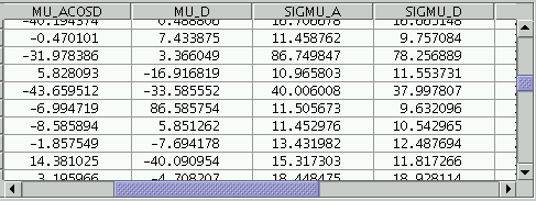
An example JTable
Many of the windows, including the Data Window, display their data in a visual component called a JTable. This displays a grid of values, with headings for each column, in a window which you can scroll around. Although JTables are used for a number of different things (for instance, showing the table data themselves in the Data Window and showing the column metadata in the Columns Window), the fact that the same widget is used provides a common look and feel.
Here are some of the things you can do with a JTable:
In some cases where a JTable is displayed, there will be a menu on the menu bar named Display. This permits you to select which columns are visible and which are hidden. Clicking on the menu will give you a list of all the available columns in the table, each with a checkbox by it; click the box to toggle whether the column is displayed or not.
Editable Column Selector
Several windows in TOPCAT invite you to select a column value from one of the loaded tables by presenting a selection box like the one in the figure. Examples are the Plot and Match windows.
In the simplest case you can simply select the value from the list of columns by clicking on the down-arrow at the right and then selecting one from the drop-down list of columns which is offered. Note that only appropriate columns will be offered - for instance if a numeric value is required, string-valued columns will not be included.
Another possibility is to use the little left/right arrows on the far right to cycle through all the known columns. This can be useful in plots, for instance to see a sequence of all the available plots against a given abcissa using only one click at a time.
Finally, you can type in an expression giving the required value. This can either be the name of a column just as if you had selected it from the drop-down list, or an expression based on column names, or even a constant value. The syntax of the expression language is explained in Section 7. Typing the column name rather than selecting it may be more convenient if the selection list is very long; typing an expression obviously gives you a lot more possibilities.
If you start typing into the box, a drop-down list of suitable columns that match what you've typed so far (autocomplete) will appear below it. You can either continue typing and hit return, or select one of the items from the drop-down list using the up/down arrow keys or the mouse.
Note that depending on your platform the selection box may not look exactly like the figure above. However, if you can type into it (probably by clicking on it) then you should be able to use expressions as described above. Some selectors however only take column names; if you can't type a value into it, you have to choose one of the options given.
The STILTS button ( ) available in several windows
opens a window displaying the command you would have to issue to the
STILTS
package to replicate the action of the current window.
Its text is continually updated to reflect the current state of the window.
) available in several windows
opens a window displaying the command you would have to issue to the
STILTS
package to replicate the action of the current window.
Its text is continually updated to reflect the current state of the window.
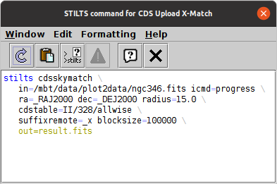
STILTS window for the CDS Upload X-Match window
STILTS is a command-line interface to much of the same functionality
that TOPCAT provides from a Graphical User Interface.
It is fully documented in its manual,
but if you don't want to read that, you can set up the action you
want in a TOPCAT window, hit the STILTS button,
and copy/paste the displayed text into the shell or a script.
Depending on configuration, the command may end with a parameter setting like
"out=result.fits", which writes the result to the named file.
You can change the filename, remove that parameter setting to display the
results directly to standard output,
or replace it with settings to postprocess the results using the extensive
pipeline processing
offered by STILTS.
TOPCAT itself contains the STILTS application, so you don't
need to install any additional software to use it.
You can run it by adding the "-stilts" flag
to a topcat command, or on a Unix-like OS use the stilts
script. If you don't already have it, you can download
stilts
to the directory containing your TOPCAT jar file;
see also SUN/256.
The Invocation formatting menu options described below
can also help.
The STILTS window button is currently available from the following windows: Match, TAP, CDS Upload X-Match, and single cone, SIA, SSA and multiple cone, SIA, SSA windows. All the Plot windows have similar functionality from their STILTS Control component.
NOTE:
The STILTS command displayed in this panel is not guaranteed
to work from the command line.
There are a few reasons for this.
The STILTS command tries to name the tables you have loaded into TOPCAT.
If they have straightforward filenames this will probably work,
but if a plotted table is for example the result of a match operation
carried out in the current session, it will not exist on disk yet
so it can't be named on the command line.
Similarly, using the names of columns or non-algebraic Row Subsets
created during the current session may result in command lines
that won't work as written,
since those values don't exist in the input files.
Constructions that may cause trouble are flagged with text in blue,
and ones that almost certainly won't work are written in red.
In this case you can prepare a table corresponding to the
current TOPCAT state, save that, and edit the STILTS command to
use the name of that file for input
(or you can reload the file and adjust the window to use that one).
Subsets as such cannot be
saved in this way, but you can achieve much the same thing by
storing subset information in a boolean column
using the To Column action ()
from the Subsets Window.
Note STILTS does not understand TOPCAT's
saved session format.
There may also be bugs in the (rather complex) command-generation code
that cause the command to fail.
Hopefully there are not too many of these,
but if you find one please report it.
The following actions are available in the toolbar:
 Update
 Copy
Copy
 Help for Command
 Show Error
The Formatting menu controls details of how the
command is laid out.
Some of these options are cosmetic, and some may need to be changed
according to your shell syntax
(the default roughly corresponds to bash).
stilts command itself is introduced.
Options are:
stilts", which will work if a
command with that name is on the execution path.
topcat -stilts", which will work
if the topcat command is on the path.
java executable
is on the path.
T" followed by the table identifier.
The identifier is the small integer shown in the table list in the
Control Window.\")
is added at the end of each line;
suitable for bash and other Unix-like shells.^")
is added at the end of each line;
suitable for Windows CMD/.bat scripts.`")
is added at the end of each line;
suitable for Windows PowerShellout=results.fits" is added to the invocation.
This isn't necessary (without it the table will be written to
standard output), but it may make it more obvious how to use the command.
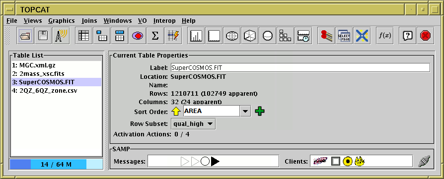
The Control Window
The Control Window is the main window from which all of TOPCAT's activities are controlled. It lists the known tables, summarises their characteristics, and allows you to open other windows for more specialised tasks. When TOPCAT starts up you will see this window - it may or may not have some tables loaded into it according to how you invoked the program.
The window consists of two main parts: the Table List panel on the left, and the Current Table Properties panel on the right. Tables loaded into TOPCAT are shown in the Table List, each identified by an index number which never changes for a given table, and a label which is initially set from its location, but can be changed for convenience.
One of the tables in the list is highlighted, which means it is the currently selected table; you can change the selection by clicking on an item in the list. Information about the selected table is shown in the properties panel on the right. This shows such things as the number of rows and columns, current sort order, current row subset selection and so on. It contains some controls which allow you to change these properties. Additionally, many of the buttons in the toolbar relate to the currently selected table.
Additionally there is a toolbar and some menus at the top which display windows and perform other actions, there is a memory monitor at the bottom left, and there may, depending on how TOPCAT was invoked, be a panel labelled SAMP at the bottom of the right hand panel.
The Table List, Current Table Properties panel, memory monitor, SAMP panel, and actions available from the Control Window's toolbar and menus are described in the following subsections.
The Table List panel on the left of the Control Window is pretty straightforward - it lists all the tables currently known to TOPCAT. If a new table is introduced by loading it from the Load Window or as a result of some action such as table joining then its name and number will appear in this list. The currently selected table is highlighted - clicking on a different table name (or using the arrow keys if the list has keyboard focus) will change the selection. The properties of the selected table are displayed in the Current Table Properties panel to its right, and a number of the toolbar buttons and menu items refer to it.
If you double-click on a table in the list, or press Return while it is selected, that table's Data Window will appear.
Certain other applications (Treeview or even another instance of TOPCAT) can interoperate with TOPCAT using drag-and-drop, and for these the table list is a good place to drag/drop tables. For instance you can drag a table node off of the main panel of Treeview and drop it onto the table list of TOPCAT, and you will be able to use that table as if it had been loaded from disk. You can also paste the filename or URL of a table onto the table list, and it will be loaded.
Sometimes while a table is being loaded a greyed-out entry will appear in this list with text like "Loading SAMP table" or similar. Such entries cannot be selected, but they let you know that something is happening.
The Current Table Properties panel on the right hand side of the Control Window contains a number of controls which relate to the currently selected table and its Apparent properties; they will be blank if no table is selected. Here is what the individual items mean:
OK
INFO/@name="QUERY_STATUS" VOTable nodes is summarised here,
in accordance with the
DALI standard).
) can be used to add
more selectors; ones further right are used only if several rows
have the same value for expressions to the left.
The Remove button if present can be used to remove
the currently least-significant selector.
Activation Actions toolbar button to
open the Activation Window.
Control Window Memory Monitor
The memory monitor is a small widget at the bottom left of the Control Window which gives an indication of TOPCAT's memory usage. The numbers indicate the currently used and maximum heap size that Java will use (e.g. "64 M" for 64 megabytes), and the two darker colours filled in from the left indicate the current total and used proportions of this. It's not necessary to understand in detail what these mean, but if the darkest (used) colour comes to fill up the whole area, the application will slow down and then signal an Out Of Memory Error. See Section 10.4 for some tips on what to do if this happens.
If you click on the memory monitor, you will request that the Java Virtual Machine performs a garbage collection round, which may have the effect of reclaiming some memory and modifying the current usage. This is not really useful (Java will garbage collect at sensible times without prompting), but you can do it if you're bored.

Control Window SAMP Panel
If TOPCAT is running in SAMP mode, the SAMP panel at the bottom of the Control Window gives a quick view of the current status of SAMP communications. For a discussion of the whats and whys of SAMP, see Section 9. Note that if not running in SAMP mode (e.g. if in PLASTIC or no-server mode) this panel will not appear. SAMP mode is the default under normal circumstances.
The panel is made up of the following main parts:
More detail and control for the information presented in this panel is available in the SAMP Window.
There are a number of buttons on the Control Window's toolbar; these are the most convenient way of invoking most of TOPCAT's functions. They are grouped as follows:
Load Table
Save Table(s)/Session
Broadcast Table
Data Window
Parameters Window
Columns Window
Subsets Window
Statistics Window
Activation Window
Histogram Plot
Plane Plot
Sky Plot
Cube Plot
Sphere Plot
Corner Plot
Time Plot
Pair Match Window
TAP Query
CDS Upload X-Match
Available Functions
 Global Variables
Help
Exit
Global Variables
Help
Exit
This section describes actions available from the Control Window menus additional to those also available from the toolbar (described in the previous section) and those common to other windows (described in Appendix A.1.2).
The File menu contains the following additional actions:
Duplicate Table
 Discard Table(s)
Send Table to ...
Discard Table(s)
Send Table to ...
 View Log
Reset Authentication
View Log
Reset Authentication
The Views menu contains actions for launching the windows which give certain views of the table metadata. Most of these are provided as toolbar buttons as well, but one is rather special-interest, so appears only in this menu:
 Datalink Window
The Graphics menu contains actions for launching the windows which give various plotting and visualisation options. The most important ones are provided as toolbar buttons as well, but this menu contains some actions not available elsewhere. The ones marked "(old)" are the plotting windows that were available before TOPCAT version 4; they have a different user interface, are generally less powerful, and are somewhat deprecated, but still work.
 Histogram Plot (old)
 2D Plot (old)
 3D Plot (old)
 Sphere Plot (old)
 Stacked Line Plot (old)
 Density Map (old)
The Joins menu contains actions for various types of table join. The items provided additional to those on the toolbar are:
Concatenation Window
 Multiple Cone Search
 Multiple SIA
 Multiple SSA
Internal Match
Multiple SSA
Internal Match
 N-Table Match
The Windows menu contains actions for controlling which table view windows are currently visible on the screen. If you have lots of tables and are using various different views of several of them, the number of windows on the screen can get out of hand and it's easy to lose track of what window is where. The actions on this menu do some combination of either hiding or revealing all the various view windows associated with either the selected table or all the other ones. Windows hidden are removed from the screen but if reactivated (e.g. by using the appropriate toolbar button) will come back in the same place and the same state. Revealing all the windows associated with a given table means showing all the view windows which have been opened before (it won't display windows which have never explicitly been opened).
)
on menus on all other windows is also useful for window management -
it brings back the control window if it's been hidden.
The VO menu groups together those actions which access remote data sources. All of these options can also be found in either the Load Window toolbar or the Joins menu.
The Interop menu contains options relevant to SAMP (or possibly PLASTIC) tool interoperability; see Section 9:
SAMP Window
Stop Internal Hub
Broadcast Table
Send Table to ...
Many of the windows you will see within TOPCAT display information about a single table. There are several of these, each displaying a different aspect of the table data - cell contents, statistics, column metadata etc. There is one of each type for each of the tables currently loaded, though they won't necessarily all be displayed at once. The title bar of these windows will say something like TOPCAT(3): Table Columns, which indicates that it is displaying information about the column metadata for the table labelled "3:" in the Control Window.
To open any of these windows, select the table of interest in the Control Window and click the appropriate toolbar button (or the equivalent item in the Table Views menu). This will either open up a new window of the sort you have requested, or if you have opened it before, will make sure it's visible.
If you have lots of tables and are using various different views of several of them, the number of windows on the screen can get out of hand and it's easy to lose track of what window is where. In this case the Control Window's Windows menu (described in Appendix A.2.6), or the Window|Control Window menu item in any of the view windows can be handy to keep them under control.
The following sections describe each of these table view windows in turn.
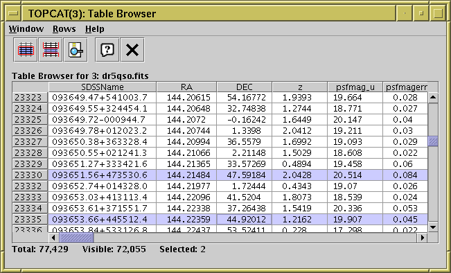
Data Window
The Data Window presents a JTable
containing the actual cells of the
Apparent Table.
You can display it using the Table Data ()
button when the chosen table is selected in the
Control Window's Table List.
You can scroll around the table in the usual way. In most cases you can edit cells by double-clicking in them, though some cells (e.g. ones containing arrays rather than scalars) cannot currently be edited. If it looks like an edit has taken place, it has.
There is a grey column of numbers on the left of the JTable which gives the row index of each row. This is the value of the special Index column, which numbers each row of the original (not apparent) table starting at 1. If the table has been sorted these numbers may not be in order.
The status line at the bottom displays three row counts:
Note that reordering the columns by dragging their headings around will change the order of columns in the table's Column Set and hence the Apparent Table.
If you have a table with very many columns it can be difficult to scroll the display sideways so that a column you are interested in is in view. In this case, you can go to the Columns Window and click on the description of the required column in the display there. This has the effect of scrolling the Data Window sideways so that your selected column is visible in the centre of the display here. To make it easier to find the required column in the Columns Window you can sort the items by column Name, UCD, Units etc first by clicking on the relevant header.
The following buttons are available in the toolbar:
Subset From Selected Rows
Subset From Unselected Rows
 Search Column
The Rows menu additionally contains the following item:
 Highlight Subset
As well as the normal menu, right-clicking over one of the columns in the displayed table will present a Column Popup Menu, which provides a convenient way to do some things with the column in question:
Replace Column
New Synthetic Column
Hide
Search Column
 Explode Array Column
float[] representing magnitudes in 5 different bands,
selecting this option will hide PMAG and insert 5 new
Float-type columns PMAG_1...PMAG_5 in its place,
each containing one of the magnitudes.
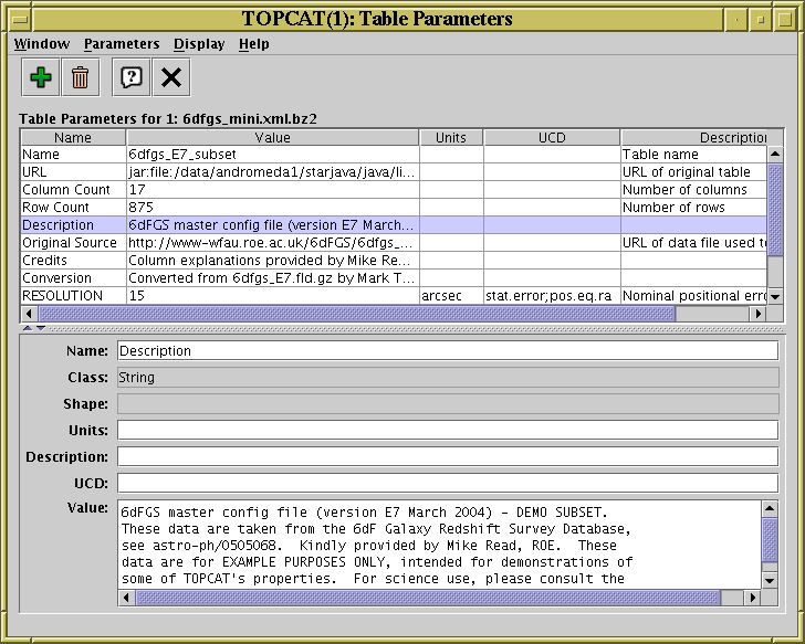
Parameters Window
The Parameters Window displays metadata which applies to the whole table
(rather than that for each column).
You can display it using the Table Parameters ()
button when the chosen table is selected in the
Control Window's Table List.
In table/database parlance, an item of per-table metadata is often known as a "parameter" of the table. At least the number of rows and columns will be listed. Some table file formats (for instance VOTable and FITS) have provision for storing other table parameters, while others (for instance CSV) do not. In the latter case there may not much much of interest displayed in this window.
The top part of the display is a JTable with one row for each parameter. It indicates the parameter's name, its value, the type of item it is (integer, string etc) and other items of interest such as units, dimensionality or UCD if they are defined. If a column of the table has no entries (for instance, the Units column might be empty because none of the parameters has had units defined for it) then that column may be absent from the display - in this case the Display menu can be used to reveal it.
You can interact with this JTable in the usual ways, for instance dragging columns sideways, changing their widths, and sorting the entries by clicking on the headings.
You can edit some parameter values and descriptions by double-clicking on them as usual.
The bottom part of the display gives an expanded view of a selected parameter (click on a row in the top part to select one). This is especially useful if the parameter value is too long to show fully in the table display. In most cases you can edit the fields here to change the value and other characteristics of a parameter.
The following items are available in the toolbar:
Add Parameter
Remove Parameter
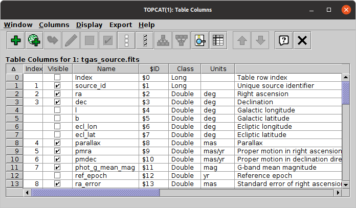
Columns Window
The Columns Window displays a JTable
giving all the information (metadata)
known about each column in the table.
You can display it using the Column Info ()
button when the chosen table is selected in the
Control Window's Table List.
The display may take a little bit of getting used to, since each column in the main data table is represented by a row in the JTable displayed here. The order and widths of the columns of the JTable widget can be changed in the same way as those for the Data Window JTable, but this has no effect on the data.
The column on the left labelled Visible
contains a checkbox in each row (one for each column of the data table).
Initially, these are all ticked.
By clicking on those boxes, you can toggle them between ticked and
unticked. When unticked, the column in question will become hidden.
The row can still be seen in this window, but the corresponding data
column is no longer a part of
the Apparent Table, so will not be seen
in the Data Window or appear in
exported versions of the table.
You can tick/untick multiple columns at once by highlighting a set of
rows by dragging the mouse over them and then using the
Hide Selected () or
Reveal Selected ()
toolbar buttons or menu items.
If you want to hide or reveal all the columns in the table, use the
Hide All () or
Reveal All () buttons.
If you select one of the JTable rows by clicking on it, the table view in the Data Window will be scrolled sideways so that the corresponding data column is visible in (approximately) the middle of the screen. This can be a boon if you are dealing with a table that contains a large number of columns.
Each column in the displayed JTable corresponds to one piece of information for each of the columns in the data table - column name, description, UCD etc. Tables of different types (e.g. ones read from different input formats) can have different categories of metadata. By default a metadata category is displayed in this JTable if at least one table column has a non-blank value for that metadata category, so for instance if no table columns have a defined UCD then the UCD column will not appear. Categories can be made to appear and disappear however by using the Display menu. The metadata items are as follows:
You can edit most of these items, e.g. to rename a column or change the expression defining a synthetic column, by double-clicking on them as usual.
By default, the order in which the rows are displayed is determined by the table's current Column Set. However, you can change the display order in this window by clicking on the column headers (in the same way as for some other JTables). The little up arrow at the top left of the scrolled JTable display indicates that the display is in its "natural" (Column Set) order, but by clicking on headers you can sort by column name, units UCD etc. Clicking sorts up, clicking again sorts down, and a third time (or clicking on the top left) restores natural order.
You can change the order of the columns in the Column Set by dragging the grey number cell at the left of the corresponding row up or down. Note however this is only possible for non-hidden columns, and it only works if this JTable is currently displayed either in its natural order or sorted by the Index column (see above) - dragging rows wouldn't have any effect if some other sort order was active. An alternative way to change Column Set order is to drag the column headers left or right in the Data Window.
A good way to find a column in the Data window if your table is too wide to do it by browsing is to sort the table in this window on some suitable item (e.g. Name, Units, UCD), scroll to the column of interest, and then click on it; that causes the view in the Data Window to scroll sideways so that the selected column is visible.
The following buttons are available in the toolbar:
New Synthetic Column
Add Sky Coordinate Columns
Replace Column With Synthetic
 Edit Column Definition
Hide Selected Column(s)
Reveal Selected Column(s)
Hide All Columns
Reveal All Columns
Explode Array Column
Edit Column Definition
Hide Selected Column(s)
Reveal Selected Column(s)
Hide All Columns
Reveal All Columns
Explode Array Column
float[] representing magnitudes in 5 different bands,
then selecting it and hitting this button will hide PMAG and
insert 5 new Float-type columns PMAG_1...PMAG_5
in its place each containing one of the magnitudes.
If the column does not have a fixed number of elements listed in
the Shape column of this window, this button is disabled.
In that case, if you know how many columns you want to explode it into,
you can enter that value into the Shape field by double-clicking on it.
This will only work for columns that are actually arrays.
 Collapse Columns to Array
double[],
and blank values in the input columns will show up as blank
array elements (NaNs).
Currently, the elements in the output column will appear in the
order of the input columns' appearance in the table,
regardless of the current ordering of the rows in this window;
the new column's Description text lists the input columns in order,
if there are not too many.
The effect is more or less the opposite of the Explode option above.
Search Column
Import as Table
Several of these actions operate on the currently selected column or columns. You can select columns by clicking on the corresponding row in the displayed JTable as usual.
As well as the normal menu, right-clicking over one of the columns in the displayed table will present a Column Popup Menu, which provides a convenient way to do some things with the column under the mouse cursor:
Search
Hide
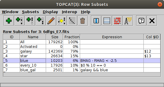
Subsets Window
The Subsets Window displays the
Row Subsets
which have been defined.
You can display it using the Row Subsets ()
button when the chosen table is selected in the
Control Window's Table List.
Two special subsets are always present: All includes the whole table, and Activated contains a single row if one has been activated by clicking on a row or point that corresponds to it.
The subsets are displayed in a JTable widget with a row for each subset. You can interact with this JTable in the usual ways, for instance dragging columns sideways, changing their widths, and sorting the entries by clicking on the headings.
The columns of the JTable are as follows:
Note: in previous versions of TOPCAT the hash sign ("#") was used instead of the underscore for this purpose; the hash sign no longer has this meaning.
 ) button described below.
Entries in the Name and Expression columns can be edited by double-clicking on them in the normal way.
The following toolbar buttons are available in this window:
New Subset
Add Sample Subset
Add Head Subset
Add Tail Subset
Edit Subset
Invert Subset
 Classify By Column
Remove Subset
To Column
Highlight Subset
Count Rows
Broadcast Subset
Classify By Column
Remove Subset
To Column
Highlight Subset
Count Rows
Broadcast Subset
The following additional menu items are available:
Send subset to ...
 Autocount rows
)
button is hit or if TOPCAT finds out the size as the result of some
other operation (such as plotting).
Autocount rows
)
button is hit or if TOPCAT finds out the size as the result of some
other operation (such as plotting).
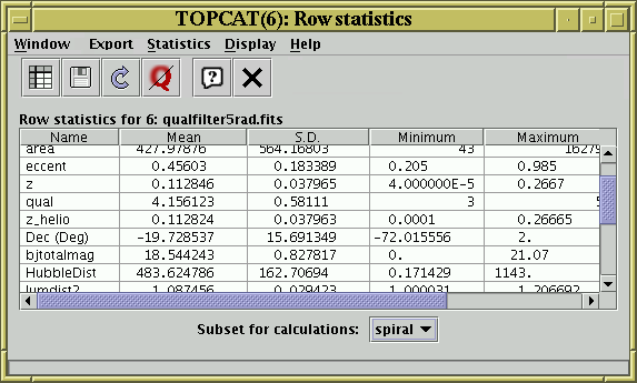
Statistics Window
The Statistics Window shows statistics for the values in each
of the table's columns.
You can display it using the Column Statistics ()
button when the chosen table is selected in the
Control Window's Table List.
The calculated values are displayed in a JTable widget with a row for each column in the main table, and a column for each of a number of statistical quantities calculated on some or all of the values in the data table column corresponding to that grid row.
You can interact with this JTable in the usual ways, for instance dragging columns sideways, changing their widths, and sorting the entries by clicking on the headings.
The following columns are shown by default:
median(abs(x-median(x)).
This is a robust measure of statistical dispersion.
Some of these quantities are suitable only for array-valued columns, and calculate per-element array statistics that are arrays of the same length as the input values (the input arrays must all be the same length):
In addition, some quantile values can calculated on demand (by selecting their values in the Display menu, as for the previous list). The available values are:
 ) option.
The quantities displayed in this window are not necessarily those for the entire table; they are those for a particular Row Subset. At the bottom of the window is the Subset For Calculations selector, which allows you to choose which subset you want the calculations to be done for. By clicking on this you can calculate the statistics for different subsets. When the window is first opened, or when it is invoked from a menu or the toolbar in the Control Window, the subset will correspond to the current row subset.
The toolbar contains the following extra buttons:
Save as Table
Import as Table
Recalculate
Approximate Quantile Calculation
For a large table the calculations may take a little while. While they are being performed you can interact with the window as normal, but a progress bar is shown at the bottom of the window. If you initiate a new calculation (by pushing the Recalculate button or selecting a new subset) or close the window during a calculation, the superceded calculation will be stopped.
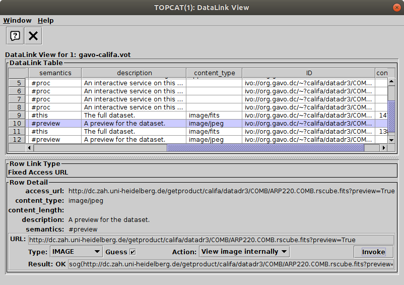
DataLink Window
The DataLink Window, unlike the other Table View Windows, is rather specialist, and only applies to a particular type of table, namely the {links}-response table format defined by the DataLink standard. This format is sometimes loosely known as the DataLink format, and is used to represent links of various kinds to external data resources.
Because of its specialist nature, this window
does not appear in the Control Window toolbar
like the other view windows, so to open it you have to
select the DataLink View item
from the Views menu in the
Control Window.
This menu item will only be enabled if the loaded table looks
like it has the appropriate form.
The upper panel of this window displays the table content just like the Data Window, but the lower panel contains link-specific information about the row that is currently selected in the upper one.
The Row Link Type sub-panel reports what type of link the given row represents. Its value depends on which table columns are filled in, and may be one of:
access_url column.
service_def column, with parameters
supplied by other columns and/or user interaction.
error_message column
indicating why a requested link cannot be supplied.
The Row Detail panel provides additional information on the row. For the rows that actually represent a link, information such as link semantics and resource content type are listed where available, along with a URL sub-panel as below.
The URL sub-panel, if present, shows the actual link URL and provides options to invoke it, i.e. to do something with the listed resource. The parts of this panel are:
In the case of a Service Invocation link type, there may be user-supplied parameters for the link. If so, a Parameters sub-panel appears at the bottom with a list of the available parameters (defaults may or may not be present) to allow you to enter values. Note that the user interface for supplying these parameters is currently very basic, and may be improved in future releases.
This section describes the plotting windows introduced at TOPCAT version 4. These provide most of the same functionality as the old-style plot windows, but additionally much more flexibility, configurability, extensibility and better performance and capabilities for making visual sense of very large data sets.
TOPCAT has a number of windows for performing data visualisation of various kinds. These share various characteristics which are described in the first subsection below; the specific windows themselves are described in the later subsections.
Seven plot windows are currently available:
More may be introduced in future releases.The rest of this section describes the plotting functions in detail.
A brief summary of improvements these windows offer over the old-style plot windows is:
The new windows allow you to assemble a stack of layers representing different plot types of different data sets on the same axes. The user interface for controlling this is quite a bit different than for the old-style plot windows, and is described in the subsequent sections. However, making a simple plot is still simple: select a table, select the columns, and you're off.
Some features from the old-style plots that are not currently available in the new-style plots are:
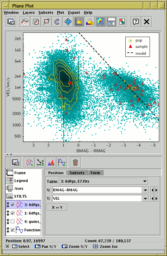
Plot window
Plot windows consist of two main parts:
the Plot Panel containing the actual plotted graphics
(by default, at the top),
and the Control Panel (by default, at the bottom).
The Control Panel is where you configure what will be plotted.
For a simple scatter plot it may just be a case of selecting what
columns to plot against each other, but it can get quite detailed.
If you want more screen space to play with, it can be helpful
to float the control panel into a separate window using the
Float Controls ( ) toolbar button;
you can find this button in both the main and the control panel toolbars.
To unfloat the control panel, either just close the control panel window,
or click the Float Controls toolbar button again.
With floating controls, the window looks like the following figure.
) toolbar button;
you can find this button in both the main and the control panel toolbars.
To unfloat the control panel, either just close the control panel window,
or click the Float Controls toolbar button again.
With floating controls, the window looks like the following figure.
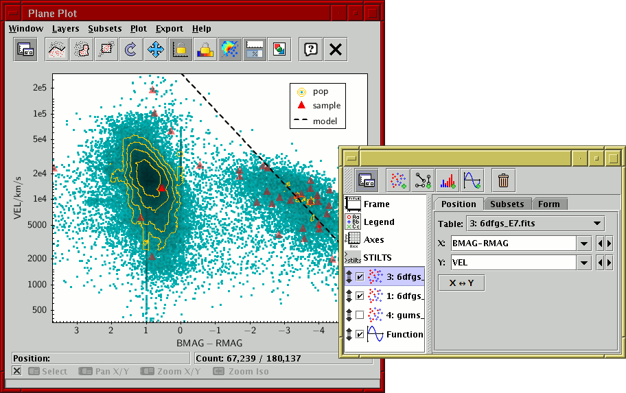
Plot window with floated control panel
The control panel itself has two main parts: a control stack on the left containing currently active controls (represented by names and icons), and a detail panel on the right which shows information about the currently selected control. Click on one of the control entries on the left to see its details on the right. Different controls have different detail panels, but in general each one will have multiple tabs for configuring different things. You can select these by clicking on the tab names. A good way to learn about the options is to click on the different controls and their tabs to see what's available and experiment with the various options to see what happens to the plot, but all the panels and tabs are also explained in this manual. The control panel also has a toolbar at the top, used for adding and removing controls from the stack.
The control list has two types of entry:
 ),
Legend (
),
Legend ( ),
Axes (
),
Axes ( ) and
STILTS () are visible.
) and
STILTS () are visible.
The different fixed controls are described in Appendix A.4.3.
) button in the
toolbar. You can also use the Layers menu at the top
of the main window to add and remove layers.
The checkbox beside each control determines whether it is currently active; if unchecked, any plotting instructions is contains will be ignored. You can set them active or inactive by clicking on the checkboxes.
You can also drag each control up or down by dragging with the
grab handle ( ). Layers lower down the list are plotted
later (perhaps obscuring earlier one), so you can drag them up and
down until you have the layers you want on top.
). Layers lower down the list are plotted
later (perhaps obscuring earlier one), so you can drag them up and
down until you have the layers you want on top.
The different layer controls are described in Appendix A.4.4.
In the foot of the window, there are also four other small panels:
 button
will make this panel go away.
button
will make this panel go away.
 )
button in the toolbar. It's nice to know that something's going on,
but it can be distracting; displaying progress also slows the plot down
a bit.
)
button in the toolbar. It's nice to know that something's going on,
but it can be distracting; displaying progress also slows the plot down
a bit.
The main toolbar at the top of the window contains the following actions (repeated in the menus):
Float Controls
Draw Subset Blob
Subset From Visible
Replot
 Rescale
 Lock Axes
 Lock Aux Range
It also affects some other dynamic ranging calculations such as Auto-Scale sizes for plot forms Size, SizeXY, Vector, SkyVector, Ellipse, SkyEllipse, XYCorr and SkyCorr.
 Sketch Frames
Replot on Data Change
) button,
or by doing anything else that would cause a replot
such as a drag/zoom action.
Sketch Frames
Replot on Data Change
) button,
or by doing anything else that would cause a replot
such as a drag/zoom action.
 Export Plot
The window menus offer an alternative way to perform the actions available from the toolbar described above. They also provide some additional options:
)
the currently selected control.
Show Plot Progress
 Show Navigation Graphics
Export Plot
STILTS Command Window
Layer Data Import
Layer Data Save
Show Navigation Graphics
Export Plot
STILTS Command Window
Layer Data Import
Layer Data Save
The following subsections explain some other features common to all the plotting windows.
All the plot windows are interactive, and you can navigate around them using the mouse buttons. For most plot types the left and right buttons and the mouse wheel do something; in 3d plots the middle button is used as well.
The details of what mouse actions do what depend on which plot window you are using, and they can also be configured to some extent using the Navigation tab in the Axes fixed control in the control stack. However, as a rule, the actions when used on the body of the plot are these:
 Left drag
 Right drag
 Middle drag
 Mouse wheel
 Left click
Most of these actions give you some visual feedback on the screen,
showing a rectangle or some arrows to give you a clue what you're doing.
If you find that distracting, you can turn it off using the
Plot|Show Navigation Graphics () menu item.

Navigation help panel at the bottom of plot windows
In each plot window there is a row at the bottom of the window
giving hints on the currently available navigation actions.
The little icons are each supposed to represent either a
click () or a drag ()
with one of the three buttons pressed,
or a wheel spin (),
and are followed by a short description of what it will achieve.
Note these hints change according to where the mouse is currently
positioned on the screen.
Moving the button over this panel will give you some help on the help.
Clicking the button will make the line disappear,
and you can bring it back with the Window|Show Navigation Help
( ) menu item.
The
) menu item.
The  button will bring up a help window specific to
the navigation in this window.
button will bring up a help window specific to
the navigation in this window.
If you are using a mouse with fewer than three buttons or no wheel, the following subsitute gestures can usually be used:
Left button
 Right button
 Middle button
Wheel
Middle button
Wheel
Most, but not all, of the available layer controls are concerned with plotting table data in some way or other. In general, these allow you to set up a way to generate a plot layer (some generated graphics) from some selected columns of a given table with a chosen style.
However, if you have more than one Row Subset for a given table, a single control can be used to generate several layers, one for each subset. In most cases it makes sense to have the graphics generated by the different subsets configured similarly, but still visually distinguishable.
These table layer controls generally have three tabs: Position, Subsets and Form. The Position tab is for specifying coordinates, and depends on the specific type of the plot and the layer control. The Subsets and Form tabs control which row subsets are plotted and how they are displayed, and a description of how they are arranged follows below.
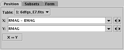
Position tab of a table data layer control
The Position tab lets you specify a table and a basic set of coordinates for the positions to plot. The details of how the data point at each of those positions is represented, including in some cases more coordinate values (e.g. for error bar sizes etc), are specified in the other tabs (usually Form).
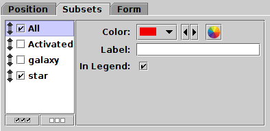
Subsets tab of a table data layer control
The Subsets tab lists the defined Row Subsets for the table you have selected in the Position tab (see the Subsets window). The subsets All and Activated are always present; others may or may not be depending on whether any have been defined. Note that actions you take in the plot (for instance selecting a new subset by region) can result in new entries being added to this list.
The list on the left names the subsets with an activation checkbox and a grab handle; the panel on the right gives the detail for the currently selected subset. Select a subset to see/change its detail by clicking on it.
For each subset you can select:
 /
/ ) buttons at the bottom of the list
can be used as a convenience to make all the subsets visible or invisible
at once (which might be useful if you have lots of subsets).
) buttons at the bottom of the list
can be used as a convenience to make all the subsets visible or invisible
at once (which might be useful if you have lots of subsets).
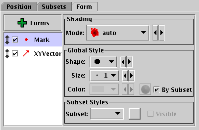
Form tab of a table data layer control
The Form tab lets you control how the data coordinates
specified in the Position tab will be used to
generate graphics on the screen.
On the left is a stack of different Form types that will each be plotted;
a default item Mark is usually included to start with,
but you can add more from the Forms menu button.
Each form in this stack can be turned on or off individually by clicking
its activation checkbox, dragged up and down using its grab handle,
or deleted using the Remove Selected Form
item from the Forms menu.
When you select a form by clicking on it in the stack, a configuration sub-panel will appear on the right hand side of this panel. This allows you to select style information to determine the details of how the plot will look for each layer, and sometimes also reports information calculated by the plot. The details differ greatly between forms, but they generally contain two sub-panels for defining the style details, Global Style and Subset Styles:
The plot windows can be used to define new Row Subsets by indicating a screen region containing the points of interest. Depending on the type of plot, one or more of the following options will be available as toolbar/menu items:
Subset From Visible Algebraic Subset From Visible Draw Blob Subset Draw Algebraic SubsetIn all these cases, when you have graphically specified a region, a dialogue box will pop up to ask you the name of the corresponding subset(s). As described in Section 3.1.1, it's a good idea to use a name which is just composed of letters, numbers and underscores. You can optionally select a subset name which has been used before from the list, which will overwrite the former contents of that subset. When you enter a name and hit the OK button, the new subset will be created and added to the list shown in the Subset Window, and the points in it will be shown straight away on the plot using a new symbol. As usual, you can toggle whether the points in this subset are displayed using the Subsets tab in the table layer control.
The different options for making these graphical selections are described in the following subsections.
The Subset From Visible ()
toolbar button creates a new subset containing all of the points
that are visible on the current plot.
When you click the button, you will be asked for a name
for the new subset.
This option can be useful if you have panned, zoomed, set the axes manually, or otherwise navigated the plot so that only the points currently visible are the ones you are interested in. However, it is only suitable if the group you are interested in corresponds to a rectangular region in the plotting space.
The Algebraic Subset From Visible
() action
(available in the Subsets menu of the
Plane and Cube
plot windows)
creates subsets containing all of the points that are visible
on the current plot.
The subset content of this is the same as for the
Subset From Visible action,
but this action defines the subset as an algebraic expression
based on the axis limits
rather than just marking the points that can currently be seen.
This can be more useful, for instance if you want to use the
subset definition in some other context.
However, it is only available for some plot types (Plane and Cube),
since in other cases the rectangular visibility
region does not correspond to a straightforward algebraic expression.
When you hit this button, the Multi Algebraic Subset Window will be displayed, showing the algebraic function(s) corresponding to the currently visible region, and offering to create a new subset (or, if there are multiple datasets plotted, several new subsets) from it.
The Draw Blob Subset ()
button allows you to draw a freehand region or regions on the plot
containing the points you are interested in.
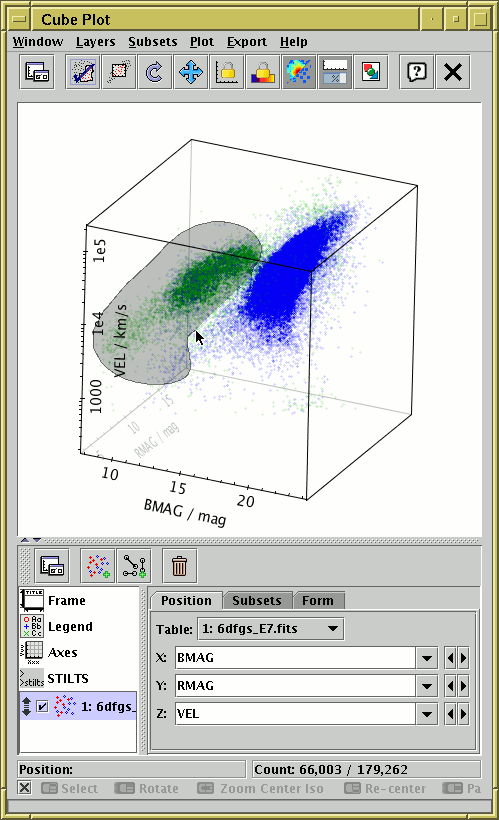
Defining a subset by blob drawing
When you click the toolbar button it will appear with a checkmark
over it ( ) to indicate that you are in
blob-drawing mode.
You can then drag the mouse around on the plot
(keep the left mouse button down while you move)
to enclose the points that you're interested in.
As you do so, a translucent grey blob will be left behind -
anything inside the blob will end up in the subset.
You can draw one or many blobs, which may be overlapping or not.
If you make a mistake while
drawing a sequence of blobs, you can right-click (or Ctrl-click)
and the most recently added blob will disappear.
When you've finished drawing your blob(s) click the
button again,
and you will be asked for a name for the subset.
) to indicate that you are in
blob-drawing mode.
You can then drag the mouse around on the plot
(keep the left mouse button down while you move)
to enclose the points that you're interested in.
As you do so, a translucent grey blob will be left behind -
anything inside the blob will end up in the subset.
You can draw one or many blobs, which may be overlapping or not.
If you make a mistake while
drawing a sequence of blobs, you can right-click (or Ctrl-click)
and the most recently added blob will disappear.
When you've finished drawing your blob(s) click the
button again,
and you will be asked for a name for the subset.
The Draw Algebraic Subset () action
allows you to select points in a region of the plot by clicking on points
of your choice to mark out a shape.
Different shapes such as polygons and circles are available,
depending on the plot type.
When complete, subsets will be defined with an
algebraic expression which you can see and edit.
This can be particularly useful
(and a better option than the blob)
if you want to refer to the subset outside of the context
of the current session,
for instance in a STILTS command or a published paper.
This action is currently only available in the Plane, Sky and Corner plot windows.
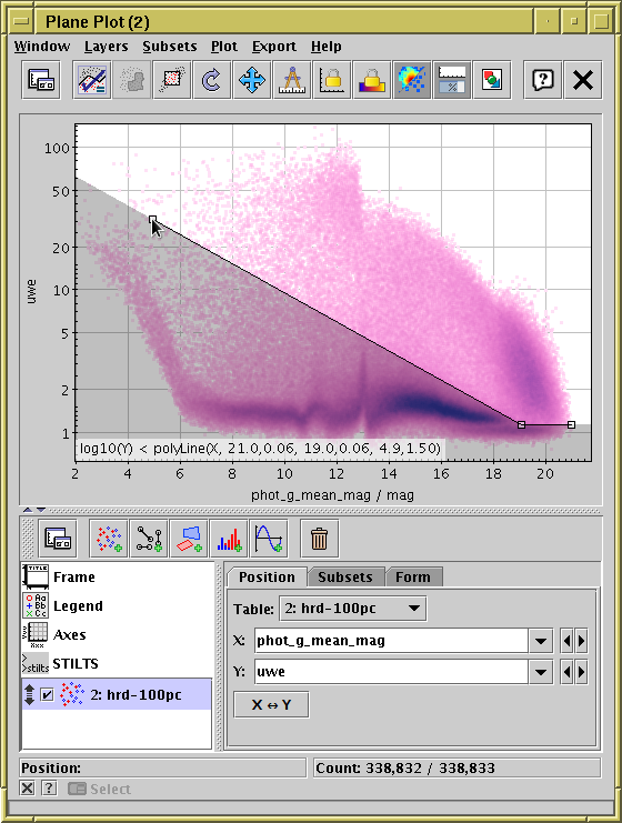
Defining a subset by algebraic drawing. This shows use of mode Below in the Plane plot.
When you use this action to define a plot region, it operates in one of a number of inclusion modes, depending on the plot type. In all cases, you click on one or more points to define the boundaries of the region. The available modes are described at the end of this section.
Operation is as follows:
button in the toolbar, and a popup window will first ask you
which inclusion mode you want to use.
Alternatively, you can use one of the mode-specific sub-menu
items in the Subsets|Draw Algebraic Subset menu
to choose a mode without the extra popup.
 ),
and a little square marker will appear near the mouse pointer
as long as it's over a suitable part of the plot.
You can then click on the plotting area to mark
the points, and the area thus defined
(according to the mode you have chosen)
will be shaded in grey.
Each point you have clicked on to define the area is marked with
the little square marker.
The algebraic form of the expression for the points entered
so far will be displayed at the bottom of the screen.
A right-click (or Ctrl-click) will remove the most recently-added point.
button again.
This will pop up the
Multi Algebraic Subset Window,
which displays the algebraic function
corresponding to the region you have outlined,
and offering to create a new subset
(or, if there are multiple datasets plotted, several new subsets)
from it.
),
and a little square marker will appear near the mouse pointer
as long as it's over a suitable part of the plot.
You can then click on the plotting area to mark
the points, and the area thus defined
(according to the mode you have chosen)
will be shaded in grey.
Each point you have clicked on to define the area is marked with
the little square marker.
The algebraic form of the expression for the points entered
so far will be displayed at the bottom of the screen.
A right-click (or Ctrl-click) will remove the most recently-added point.
button again.
This will pop up the
Multi Algebraic Subset Window,
which displays the algebraic function
corresponding to the region you have outlined,
and offering to create a new subset
(or, if there are multiple datasets plotted, several new subsets)
from it.
The generated expression tries to be as compact and comprehensible as possible. Precision of the indicated points is determined from the pixel resolution of the plot, so literal numbers are not more unwieldy than they have to be.
The available inclusion modes depend on the plot type, as follows:
isInside function.
x>x0 && x<x1 && y>y0 && y<y1.
hypot(x-x0, y-y0)<r,
using the hypot function
(hypot(x,y) = sqrt(x*x+y*y)).
square((x-x0)/a) + square((y-y0)/b)<1,
using the square function
(square(x)=x*x).
square(a(x-x0)+b(y-y0))+square(c(x-x0)+d(y-y0))<1,
using the square function
(square(x)=x*x).
y<y0, and
for two points it has the form y<m*x+c.
If there are more points, the special
polyLine function is used.
skyDistance function.
inSkyEllipse function.
inSkyPolygon function.
Cartesian axes with various scaling options are used in the Plane, Cube and Time plot windows. By default, these axes are scaled linearly, meaning a constant difference in data values maps to a constant distance on the plot axis, but other scalings can be chosen.
The available options, mapping data coordinate d to a position on the graphical axis g are:
asinh(x/a).
symlog(t,s,x).
It was copied from the
matplotlib scale of the same name.
A plot comparing these scaling functions on linear axes is shown for reference below:
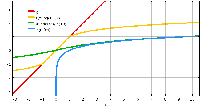
Scaling functions shown on linear axes.
These scales are selected for use in the Coords tab of the Axis Control for Plane, Cube and Time plot windows.
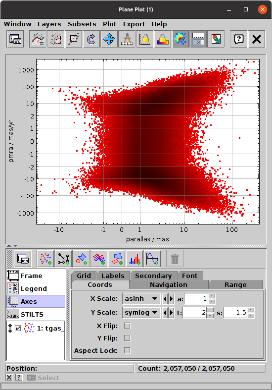
2d scatter plot using asinh and symlog axis scalings
You can select one of the options from the Scale selectors in the normal way using the drop-down list or the little left-right arrows to cycle through the choices. Some of these options (Asinh and Symlog) require parameters, and labelled entry boxes will appear next to the selector when they are selected. To adjust them you can either type in a number or use the tiny up-down arrows to step through larger or smaller values. Hovering over the entry box will pop up a tooltip explaining its meaning.
The Measure Distance ( ) action is
available from some plot windows
(Plane,
Histogram,
Sky,
Corner and
Time plots).
This allows you to use the mouse to measure the distance between
two points on the plot.
To use it, first click the Measure Distance
toolbar button or menu item,
and then press the mouse button on a point in the plot from
which you wish to measure, and drag the mouse, holding down the button,
to the point you wish to measure to.
As you drag the mouse, the distance(s) between the two points
are displayed and updated interactively.
Once you release the mouse button, measurement mode is exited,
and you need to invoke the action again to make another measurement.
) action is
available from some plot windows
(Plane,
Histogram,
Sky,
Corner and
Time plots).
This allows you to use the mouse to measure the distance between
two points on the plot.
To use it, first click the Measure Distance
toolbar button or menu item,
and then press the mouse button on a point in the plot from
which you wish to measure, and drag the mouse, holding down the button,
to the point you wish to measure to.
As you drag the mouse, the distance(s) between the two points
are displayed and updated interactively.
Once you release the mouse button, measurement mode is exited,
and you need to invoke the action again to make another measurement.
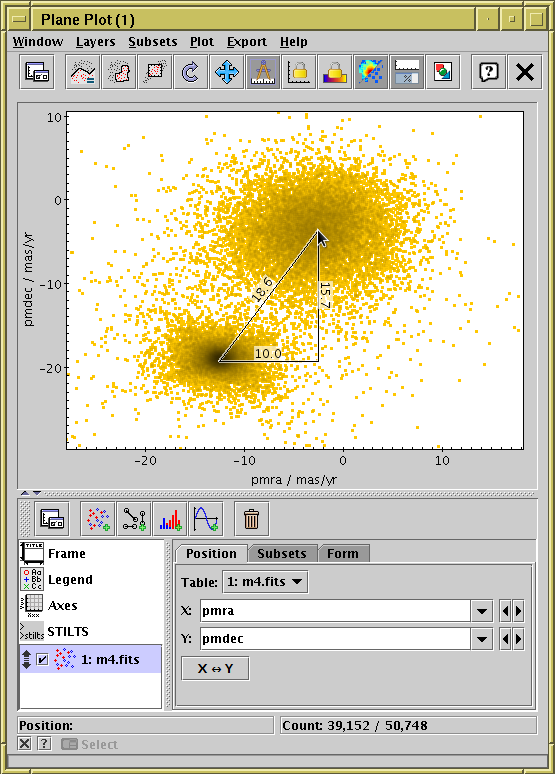
Measuring distance in the Plane Plot
The details of what distances are displayed depends on the plot window in question, according to what metrics are defined on the plot space. For the Sky plot, the shorter great circle arc is drawn on the plot between the two points, and the distance is labelled in degrees, minutes or seconds. For the Histogram and Time plots, vertical and horizontal components are drawn and labelled in terms of the distances along the corresponding axis. For the Plane plot, both components and the direct distance are measured.
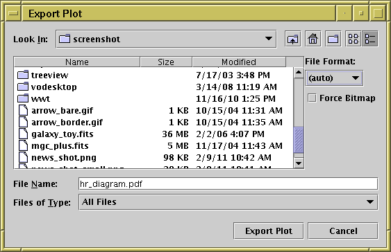
Plot export window
The Plot Export Window can be reached with the
Export plot to file ()
toolbar button in any of the plot windows.
You can select a file in the usual way, and save the plot in one of the following graphics formats:
There are two additional controls on the right hand side of this window:
Exporting to the pixel-based formats (GIF, JPEG, PNG) is fairly straightforward: each pixel on the screen appears as one pixel in the output file. PNG is generally recommended. GIF works well in most cases, but if there are more than 255 colours some of the colour resolution will be lost. JPEG can preserve a wide range of colours, but does not support transparency and is lossy, so close inspection of image features will reveal blurring.
When exporting to Portable Document Format (PDF), Scalable Vector Graphics (SVG) or Encapsulated PostScript (EPS), which are vector graphics formats, there are a few things to consider:
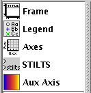
Fixed controls in control panel stack
Fixed controls are those controls that appear at the top of the stack in the control panel, and do not have a checkbox or a drag handle. They are used to configure or monitor the overall appearance of the plot, independent of any particular plot layer or data set. Those common to all plot types are described in the following subsections, though some plot types may also have their own.
The Frame control ()
controls the graphical area on which the plot graphic is drawn.
It contains two tabs, Size and Title.
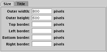
Frame control Size tab
The Size tab allows you to set the geometry of the generated plot in pixels. By default, the plot is simply resized to fit the current size and shape of the window. However, if you fill in the Outer width and/or Outer height fields, the size will instead be fixed to the given dimension in pixels. Note if you pick a large value, you may need to manually resize the window to see all of the plot. Similarly, the border fields fix the number of pixels surrounding the data region of the plot; if these are left blank, as by default, these borders are sized to accommodate the things that have to fit in them (such as axis annotations and the Aux axis colour ramp).
The main use for this tab is to fix the size and alignment of the generated images if you want to export a series of similar plots.
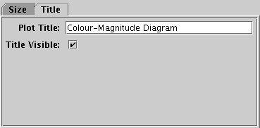
Frame control Title tab
The Title tab allows you to give a title for the plot. If text is filled in the Plot Title field, and if the Title Visible checkbox is checked, then the given text will appear at the top of the plot.
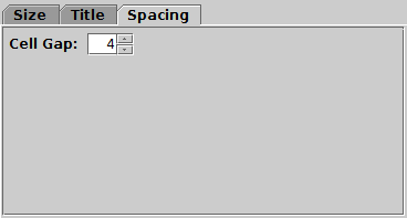
Frame control Spacing tab
For some plot types only, this tab provides options to control the spacing between elements of the plot. For the Time Plot it contains the Cell Gap option which controls the number of blank pixels between individual panels in the stack of plots. For other plot types this configuration is not relevant, or is available from the Axes control.
The Legend control ()
is always visible in the plot Control Panel.
It allows you to configure whether and how the plot legend appears.
This control has two tabs, Style and Location.
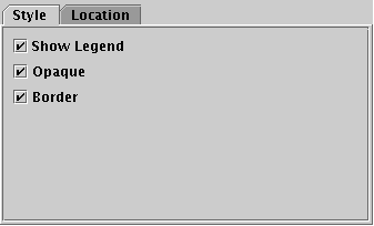
Legend control Style tab
The Style tab configures the appearance of the legend panel, and has the folowing options:
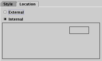
Legend control Location tab
The Location tab configures where on the plot the legend is drawn (if present). There are two options, External and Internal. If Internal is chosen, then a control is activated showing a small box inside a large box. Drag the small box around with the mouse to change the position of the legend inside the plot bounds.
Note the font used in the legend is currently controlled by the font from the Axes selector.
The Axes control ()
has a number of tabs specific to the particular plot type.
These tabs allow you to configure things like the axis ranges,
linear/log axis scaling, axis labelling, grid drawing,
details of the navigation controls and so on.
The different plot types have axis controls that differ significantly
from each other, so the specific axis controls are described separately
along with each plot type:
The STILTS control ()
displays the command you would have to issue to the
STILTS package
to reproduce the currently visible plot.
The text is continuously updated to match the currently selected
options, layers and navigation status.
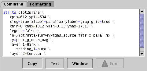
STILTS control Command tab
Unlike the other fixed controls, this one does not provide any options to change the current plot, and if you just want to use TOPCAT interactively you don't need to use it at all. But if you want to be able to regenerate the current plot from the command line or a script without setting it up again from a GUI, for instance to generate publishable figures in a reproducible way, you may find it useful.
STILTS is a command-line interface to all the functionality
that TOPCAT provides from a Graphical User Interface.
Any plot that can be displayed in TOPCAT can also be generated
by providing the right parameters to one of the STILTS
plotting commands.
The STILTS user document provides a full
tutorial introduction
for these commands, as well as detailed documentation for
each of the plotting commands
(plot2plane,
plot2sky, ...)
and many
examples.
However, there is a large number of parameters to configure,
and the command line to reproduce a complex plot can be quite lengthy,
so this control helps you to set up such plots by constructing
the command line corresponding to what you can currently see.
The text displayed in this panel can either be copied directly
to reproduce a plot you have set up interactively, or it can
be used as a basis for later adjustments to some of the parameters.
TOPCAT itself contains the STILTS application, so you don't
need to install any additional software to use it.
You can run it by adding the "-stilts" flag
to a topcat command, or on a Unix-like OS use the stilts
script. If you don't already have it, you can download
stilts
to the directory containing your TOPCAT jar file;
see also SUN/256.
The Invocation formatting options described below
can also help.
You can use this facility with very little understanding of
the details of STILTS.
You just need to copy the text
(using the Copy button or however that's usually done
on your OS)
and paste it onto a system command line or into a script.
Executing the resulting command should then pop up the current plot
in a new window outside of TOPCAT.
If it doesn't work, changing some of the Formatting
options described below
(e.g. setting Invocation to Class-path) may help.
To write the result to a graphics file instead of displaying it
in a window, just add a parameter like out=plot.png
to the end of the line.
The available graphics output formats are listed
in Appendix A.4.2.6.
To understand the generated command and get a better idea of how to tweak the parameters to adjust the plot, you can consult the STILTS user document mentioned above. Just watching how the displayed command changes as you interact with the plot is another way to learn what does what.
This display is available both as a Fixed Control and as a separate window. Both do the same thing, but the window may be convenient if you want to see the way the command text changes as you interact with the GUI in other parts of the fixed or layer controls. To pop up or hide the separate window display, you can either use the Window button at the bottom of the fixed control, or the Export|STILTS Command Window menu item.
Some actions are available from buttons or menu items:
NOTE:
The STILTS command displayed in this panel is not guaranteed
to work from the command line.
There are a few reasons for this.
The STILTS command tries to name the tables you have loaded into TOPCAT.
If they have straightforward filenames this will probably work,
but if a plotted table is for example the result of a match operation
carried out in the current session, it will not exist on disk yet
so it can't be named on the command line.
Similarly, using the names of columns or non-algebraic Row Subsets
created during the current session may result in command lines
that won't work as written,
since those values don't exist in the input files.
In this case you should prepare a table corresponding to the
current TOPCAT state, save that, and edit the STILTS command to
use the name of that file for input (or you can reload the file
and do plots using that). Subsets as such cannot be
saved in this way, but you can achieve much the same thing by
storing subset information in a boolean column
using the To Column action ()
from the Subsets Window.
Note STILTS does not understand TOPCAT's
saved session format.
There may also be bugs in the (rather complex) command-generation code
that cause the command to fail or to generate a slightly different plot.
Hopefully there are not too many of these,
but if you find one please report it.
Another thing that can cause trouble is quoted values
in algebraic expressions, since STILTS quoting syntax
does not always work well on the shell command line.
If there are quoted expressions within a quoted argument it is
sometimes helpful to escape the inner quotes,
e.g. converting
cmd_1='select "gmag > rmag"' to
cmd_1='select \"gmag > rmag\"'.
Another approach is to avoid unnecessary spaces,
which may allow inner quotes to be omitted.
An attempt is made to flag problems in the displayed command line.
Constructions that are suspected or expected to cause trouble
when executing it are highlighted in a different colour.
If the command line itself seems to violate the plotting command syntax,
the Error () button will become enabled;
clicking on it will display some indication of what's wrong.
However, the best way to test whether a displayed command will work
is to copy and paste it onto an actual command line and try to run it.
If it works, the plot will show up in a new window.
To export this into a graphic file, simply add or modify the
out parameter (e.g. out=tc-plot.pdf).
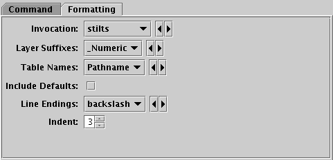
STILTS control Formatting tab
The Formatting tab gives you various options to adjust how the generated STILTS command is displayed in the Command tab. In the popup window version of this display, these options are available as items in the Formatting menu instead.
You may want to adjust these options for personal taste,
or so the output works better with the
command-line environment you're using.
The basic format is intended to work with a Unix-like shell
such as bash;
in most cases the name=value settings should
not be too sensitive to shell-specific syntax,
but it may be useful for instance to change line ending characters.
The available formatting options are:
stilts command itself is introduced.
Options are:
stilts", which will work if a
command with that name is on the execution path.
topcat -stilts", which will work
if the topcat command is on the path.
java executable
is on the path.
layer<suffix>=<layer-type>"
(see SUN/252).
You can choose any form for these suffixes that does not interfere
with the non-suffix parts of the other parameters,
and this option allows you to choose how they are generated.
Options are:
_1, _2, ..._A, _B, ..._a, _b, ...1, 2, ...A, B, ...T" followed by the table identifier.
The identifier is the small integer shown in the table list in the
Control Window.\")
is added at the end of each line;
suitable for bash and other Unix-like shells.^")
is added at the end of each line;
suitable for Windows CMD/.bat scripts.`")
is added at the end of each line;
suitable for Windows PowerShellThe Aux Axis control ( ) is only visible
when at least one layer is using the shared colour map.
The following plot layers do this:
) is only visible
when at least one layer is using the shared colour map.
The following plot layers do this:
If no layer is using the shared colour map, then this control will not appear in the stack.
When present, this control has three tabs, Map, Ramp and Range, described below.
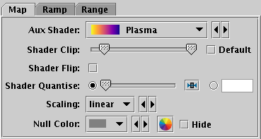
Aux axis control Map tab
The Map tab controls the aux axis colour map. It has the following options:
The default range is clipped at one end for colour maps that fade to white, so that all the plotted colours will be distinguishable against a white background. That is generally a good idea for scatter-type plots, but may not be so good for plots where the whole plotting surface is coloured in, like density maps or spectrograms, so in that case you might want to uncheck Default and leave the handles at the extreme ends of the slider.
linear
log
histogram
histolog
asinh
square
sqrt
acos
cos
linear, log, asinh,
square,
sqrt, acos and cos options
just apply the named function to the full data range,
in some cases with some normalisation.
Note that log scaling will ignore any negative values.
The histogram options on the other hand use a scaling function
that corresponds to the actual distribution of the data, so that
there are about the same number of points (or pixels, or whatever
is being scaled) of each colour.
The histogram options are somewhat more expensive,
but can be a good choice if you are exploring data whose
distribution is unknown or not well-behaved over its min-max range.
The histogram and histolog options both
assign the colours in the same way, but they display the colour
ramp with linear or logarithmic annotation respectively;
the histolog option also ignores non-positive values.
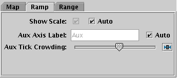
Aux axis control Ramp tab
The Ramp tab controls the display and annotation of the colour ramp that displays the colour map on the plot. It has the following options:
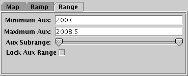
Aux axis control Range tab
The Range tab lets you enter lower and upper values for the aux data range by hand, and provides a double slider to restrict the range within these limits. If either the lower or upper range is left blank, it will be determined from the data.
The Lock Aux Range checkbox controls whether
the aux range is automatically updated as the plot is adjusted
(for instance as you navigate around it with the mouse).
If locked, the range will stay the same, but otherwise (the default)
it is dynamically updated for the current view of the plot.
This checkbox is a duplicate of the toggle button on the plot
window toolbar described in Appendix A.4.2.
Note the font used for labelling the aux axis is currently controlled by the font from the Axes selector.
The layer controls are controls in the Control Stack that can be added, removed and moved around to determine what layers go to make up the contents of a plot. You can have zero, one or several of each. Which ones are available is dependent on which plot type you are using (for instance the Spectrogram control is only available for the Time plot). Add instances of each control to the control stack by using the appropriate button from the control panel toolbar (the one in the lower half of the window) or the corresponding item in the Layers menu.
The available layer controls are described in the following subsections. More may be added in future releases.
The Position layer control ( )
is available for all the plot types
(except the Corner Plot, which uses the similar
Matrix control).
Most plots start off with one of these in the stack by default,
and you can add a new instance by using the
Add Position Control (
)
is available for all the plot types
(except the Corner Plot, which uses the similar
Matrix control).
Most plots start off with one of these in the stack by default,
and you can add a new instance by using the
Add Position Control ( ) button
in the control panel toolbar,
or the corresponding item in the Layers menu.
) button
in the control panel toolbar,
or the corresponding item in the Layers menu.
This is the control which is used for most of the data plotting in the plotting windows. Each instance of this control in the stack does plotting for a particular set of positions from a single table. The set of positions is defined in the Positions tab as a column name or expression for each plot coordinate (e.g. for X and Y in a plane plot). However, the control can generate multiple layers from these positions; the Subsets tab controls which subsets are plotted and how each one is identified, and the Form tab provides many options for what graphics will be plotted based on the positions.
This control is a Table Data control as described in Appendix A.4.2.2. That section explains the Subsets tab; the Position and Form tabs are described in more detail below.
Position tab of Position layer control, for Plane plot
In the Position tab you enter the base position coordinates for each plotted point. This generally means selecting a table and providing a value (table column or expression) for each positional coordinate. When you first open a plot window, TOPCAT gives you a table layer control by default, and attempts to fill in the positional coordinates with some reasonable values from the table (for instance the first few numeric columns).
Note the details of the Position tab will be different for different plot types, for instance the Cube plot has a Z coordinate field alongside X and Y.
For the Plane plot only, there is an X<->Y button that lets you swap the contents of the X and Y fields for convenience. Note that swapping those contents is the only thing it does, it does not for instance swap the log flags for the axes, so the result may not be exactly the same as reflecting the plot about the X=Y line.
Form tab of Position layer control
The Form tab lets you define how the specified data set is plotted. The stack on the left gives a list of forms currently being plotted, and the panel on the right shows the detailed configuration for the currently selected form.
When first added, the stack contains a single entry, Mark,
which plots a marker of a given fixed shape and size.
The colour is by default determined by the setting in the Subsets tab.
For a simple scatter plot, this is all that you need.
However, there are a number of other forms that you can plot as well
or instead of the simple markers - vectors, error bars, ellipses,
contours, text labels etc. You add a new form to the stack by
clicking on the Forms button,
which gives you a menu of all the available forms for the current layer control.
You can remove a form by selecting it and selecting
the Remove () button in the same menu.
You can also activate/deactivate the entries in the stack
with the checkbox and move them up and down with the drag handle as usual.
The list of forms that are avaiable depends on the plot type;
the full list is in Appendix A.4.5.
The detail panel of each form depends on the form itself. It is divided into the following panels, though not all forms have all the panels.
The Pair Position layer control ( )
allows you to plot symbols linking two positions in the plot space
from the same table.
You can add one of these controls to the stack by using the
Add Pair Control (
)
allows you to plot symbols linking two positions in the plot space
from the same table.
You can add one of these controls to the stack by using the
Add Pair Control ( ) button
in the control panel toolbar,
or the corresponding item in the Layers menu.
) button
in the control panel toolbar,
or the corresponding item in the Layers menu.
This control is particularly useful for visualising the results
of a crossmatch, and it is used automatically by the
Plot Result ( ) option offered by
some of the Match Window results.
If you want to plot pairs of points from different input tables,
you first have to create a joined table by using one of the
crossmatch functions.
) option offered by
some of the Match Window results.
If you want to plot pairs of points from different input tables,
you first have to create a joined table by using one of the
crossmatch functions.
It works in a similar way to the Single Position Layer Control, but the Position tab has fields for not one but two sets of coordinates to fill in.
This control is a Table Data control as described in Appendix A.4.2.2. That section explains the Subsets tab; the Position and Form tabs are described in more detail below.
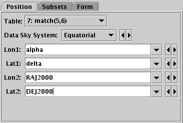
Position tab of Pair Position layer control, for Sky plot
In the Position tab you enter the pair of position coordinates for each plotted pair. This generally means selecting a table and providing a value (table column or expression) for the first and second sets of positional coordinates.
Note the details of the Position tab will be different for different plot types, for instance the Sky plot has Lon1, Lat1, Lon2 and Lat2 fields for the first and second longitude/latitude pairs, while a Plane plot has X1, Y1, X2 and Y2.
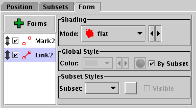
Form tab of Pair Position layer control
The Form tab lets you define how the specified data set is plotted. The list on the left gives a list of forms currently being plotted, and the panel on the right shows the detailed configuration for the currently selected form.
The available forms for a pair plot
(select them using the Forms button)
are currently
Mark2 ( )
which draws the points at both ends of the pair, and
Link2 (
)
which draws the points at both ends of the pair, and
Link2 ( )
which draws a line linking them.
You can configure these, and select them on or off, separately.
The detail panel for these forms are dependent on the form itself
and are described in more detail in Appendix A.4.5,
but the detail panels are divided into these parts:
)
which draws a line linking them.
You can configure these, and select them on or off, separately.
The detail panel for these forms are dependent on the form itself
and are described in more detail in Appendix A.4.5,
but the detail panels are divided into these parts:
The Quad Position layer control ( )
allows you to plot symbols defined by four positions in the plot space
from each row of a table - typically some kind of quadrilateral.
You can add one of these controls to the stack by using the
Add Quad Control (
)
allows you to plot symbols defined by four positions in the plot space
from each row of a table - typically some kind of quadrilateral.
You can add one of these controls to the stack by using the
Add Quad Control ( ) button
in the control panel toolbar,
or the corresponding item in the Layers menu.
) button
in the control panel toolbar,
or the corresponding item in the Layers menu.
It works like the Single Position and Pair Position Layer Controls, but the Position tab has fields for four sets of coordinates to fill in.
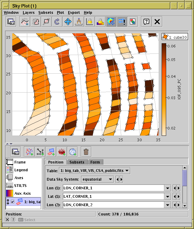
Sky Plot Window with a Quad control
This control is a Table Data control as described in Appendix A.4.2.2. That section explains the Subsets tab; the Position and Form tabs are described in more detail below.
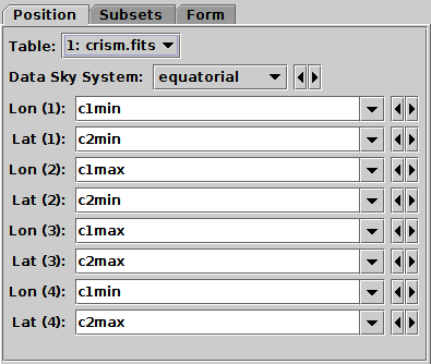
Position tab of Quad Position layer control, for Plane plot
In the Position tab you select a table and enter four sets of position coordinates (using a column name or expression for each one) to define the plotted quadrilaterals.
Note the details of the Position tab will be different for different plot types, for instance the Sky plot has Lon (1), Lat (2) etc for the (longitude,latitude) pairs, while the Cube plot has X (1), Y (1), Z (1) etc. for the 3-dimensional Cartesian triples.
In some cases, for instance EPN-TAP tables with bounding boxes in sky plots, positions will be filled in automatically. You can of course change these default selections.
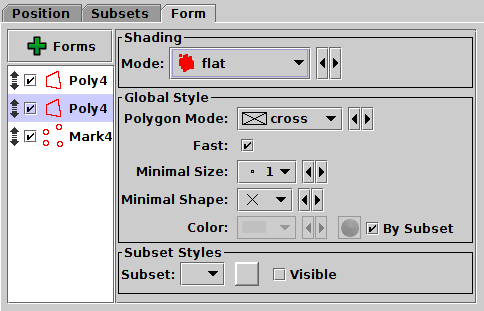
Form tab of Quad Position layer control
The Form tab lets you define how the specified data set is plotted. The list on the left gives a list of forms currently being plotted, and the panel on the right shows the detailed configuration for the currently selected form.
The available forms for a quad plot
(select them using the Forms button)
are currently
If you want to draw triangles instead of quadrilaterals, you can just supply the same coordinates for two of the positions. If you want a polygon with more vertices, try the Polygon form from the single position layer control.
The Matrix layer control ( )
is available only for the Corner Plot.
The Corner Plot window starts with one of these in the stack by default,
and you can add a new instance by using the
Add Position Control (
)
is available only for the Corner Plot.
The Corner Plot window starts with one of these in the stack by default,
and you can add a new instance by using the
Add Position Control ( ) button
in the control panel toolbar,
or the corresponding item in the Layers menu.
) button
in the control panel toolbar,
or the corresponding item in the Layers menu.
This is the control that supplies all the plots for the Corner plot. Each instance of this control in the stack does plotting for a set of multidimensional points from a single table. The set of points is defined in the Position tab as a column name or expression for each plot coordinate, while the Fill tab provides some controls that can help to fill in in the Position tab. The control can generate multiple different layers from these positions; the Form tab provides many options for what graphics will be plotted based on the positions, and the Subsets tab controls which subsets are plotted and how each one is identified.
This control is a Table Data control as described in Appendix A.4.2.2. That section explains the Subsets tab; the Position, Fill and Form tabs are described in more detail below.
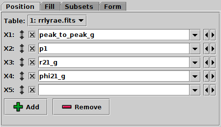
Position Tab of Matrix layer control
To select the quantities that will be plotted against each other, in the Position tab select column names or enter algebraic expressions into the fields marked X1, X2, X3 etc. Grid cells will be plotted for each distinct pair (scatter-plot-like) and single (histogram-like) combination of the specified coordinates.
This position entry panel has a few features not found in the other plot types:
)
and Remove ()
buttons can be used to increase/decrease the number of fields visible
for coordinate entry.
)
by each coordinate;
you can drag this up or down using the mouse to re-order the coordinate
values you have entered.
)
by each coordinate;
you can use this to remove the adjacent value from the plot
(all the ones below will move up one).
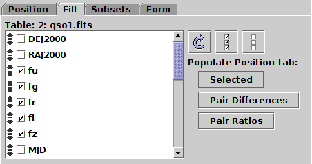
Fill Tab of Matrix layer control
The Fill tab lets you choose columns from the table you are plotting, and use them to populate the selectors in the Position tab. Moving and selecting the columns in this tab does nothing on its own, but if you hit one of the buttons under the Populate Position tab heading on the right, the Position tab, and hence the plot, is updated accordingly. This doesn't do anything that can't be done by filling in fields in the Position tab directly, but it can be a quicker and more convenient way to do it.
The left hand panel shows all the columns in the input table
(as selected in the Position tab).
They can be reordered using the mouse by dragging them with their
Grab Handle ()
and the checkbox by each one can be selected.
The three buttons at the top of the right hand panel also affect this list:
: Reloads the column list from the table;
this ensures that the order of the columns in the list
is the same as the current column order in the table it comes from
: Selects all the columns in the list
: Unselects all the columns in the list
When you have selected the columns you're interested in, you can hit one of the buttons below the Populate Position Tab heading.
A, B, C and D
are selected in the list here,
then clicking this button
will fill in the selectors in the Position tab with
X1=A-B, X2=A-C, X3=A-D,
X4=B-C, X5=B-D,
X6=C-D.
The number of replacement coordinates
(hence the linear size of the grid)
will be N(N-1)/2 so it can end up generating a lot of plots.
This is a rather special-interest option, but it can be handy
for instance when working with sets of correlated parameters
such as source magnitudes.
A/B, X2=A/C, X3=A/D,
X4=B/C, X5=B/D,
X6=C/D.
This could be useful when working with sets of fluxes.
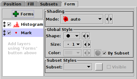
Form Tab of Matrix layer control
The Form tab lets you define how the specified data set is plotted. The stack on the left gives a list of forms currently being plotted, and the panel on the right shows the detailed configuration for the currently selected form.
When first added, the stack contains two entries,
Mark and Histogram.
This gives you a scatter plot on all the off-diagonal grid positions,
and a histogram on all the diagonal ones.
However, there are a number of other forms that you can plot as well
or instead of the simple markers;
two-coordinate plots like contours and linear fits on the off-diagonal
positions, and
one-coordinate plots like KDEs on the diagonal positions.
You add a new form to the stack by
clicking on the Forms button,
which gives you a menu of all the available forms.
You can remove a form by selecting it and clicking
the Remove () button in the same menu.
You can also activate/deactivate the entries in the stack
with the checkbox and move them up and down with the drag handle as usual.
The detail panel of each form depends on the form itself. It is divided into the following panels, though not all forms have all the panels.
The Healpix layer control ( )
is available from the Sky Plot Window
for plotting tables that represent HEALPix maps on the celestial sphere.
You can add one of these controls to the stack by using the
Add HEALPix Control (
)
is available from the Sky Plot Window
for plotting tables that represent HEALPix maps on the celestial sphere.
You can add one of these controls to the stack by using the
Add HEALPix Control ( ) button
in the control panel toolbar,
or the corresponding item in the Layers menu.
) button
in the control panel toolbar,
or the corresponding item in the Layers menu.
Each row in the table must represent a single healpix tile, and a value from that row is used to colour the corresponding region of the sky plot. The resolution (healpix order) of the input table is supplied or may be guessed in order to do the plot, but the plot may be drawn at a degraded order (bigger pixels) if required.
Note this is different from the SkyDensity form, which takes a table containing sky positions, and represents that as a density map on the healpix grid by gathering the rows up into bins. The control described here works on a table for which that binning has already been done, for instance as a prepared sky map data product, by exporting from a SkyDensity layer, or by executing a suitable (GROUP BY healpix_index) database query.
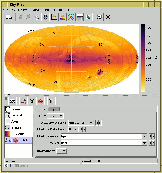
Sky Plot Window with a Healpix layer
This control has two tabs, Data and Style.
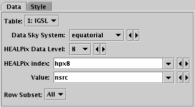
Healpix control Data tab
The Data tab lets you specify the table and columns containing the healpix tile data. It has the following fields:
$0 or $index token,
you would have to write e.g. $index-1.
To control the colour map used to colour the sky tiles,
use the Aux fixed control.
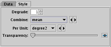
Healpix control Style tab
The Style tab lets you configure additional details of the plot's appearance. It has the following fields:
degrade>0.
For density-like values
(count-per-unit, sum-per-unit)
the scaling is additionally influenced by the
Per Unit option.
The available options are:
sum:
the sum of all the combined values per binsum-per-unit:
the sum of all the combined values per unit of bin sizecount:
the number of non-blank values per bin (weight is ignored)count-per-unit:
the number of non-blank values per unit of bin size
(weight is ignored)mean:
the mean of the combined valuesmedian:
the median of the combined values (may be slow)q1:
the first quartile of the combined values (may be slow)q3:
the third quartile of the combined values (may be slow)min: the minimum of all the combined valuesmax: the maximum of all the combined valuesstdev:
the sample standard deviation of the combined valueshit:
1 if any values present, NaN otherwise (weight is ignored)count-per-unit or sum-per-unit).
If the Combination mode is calculating values per unit area,
this configures the area scale in question.
For non-density-like combination modes
(e.g. sum or mean)
it has no effect.
The available options are:
steradian: steradiandegree2: square degreearcmin2: square arcminutearcsec2: square arcsecondmas2: square milliarcsecuas2: square microarcsecThe Histogram layer control ( ),
allows you to make a 1-dimensional histogram-like plots
(weighted and unweighted histograms, various kinds of Kernel Density Estimates).
It is the main control in the
Histogram plot window,
but is also available in the Plane
and Time
plot windows, so you can overplot a histogram on scatter or time plots,
if you can think of some reason to do that.
The Histogram window starts off with one of these controls in the stack by
default, but as usual you can add more by using the
Add Histogram Control (
),
allows you to make a 1-dimensional histogram-like plots
(weighted and unweighted histograms, various kinds of Kernel Density Estimates).
It is the main control in the
Histogram plot window,
but is also available in the Plane
and Time
plot windows, so you can overplot a histogram on scatter or time plots,
if you can think of some reason to do that.
The Histogram window starts off with one of these controls in the stack by
default, but as usual you can add more by using the
Add Histogram Control ( ) button
in the control panel toolbar,
or the corresponding item in the Layers menu.
) button
in the control panel toolbar,
or the corresponding item in the Layers menu.
Each instance of this control in the stack can make histogram-like plots of a particular quantity from a particular table. The value to be histogrammed, and optionally an associated weighting term, are defined in the Positions tab using column names or expressions. However, the control can generate multiple layers from these coordinates; the Subsets tab controls which subsets are plotted and how each one is identified, and the Form tab provides many options for what graphics will be plotted based on the sample values specified in the Position tab.
This control is a Table Data control as described in Appendix A.4.2.2. That section explains the Subsets tab; the Position and Form tabs are described in more detail below.
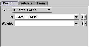
Position tab of Histogram layer control
In the Position tab you enter the value of the X value, the one whose values along the X axis will be used to generate the plots. This may be a table column name or an expression. You may also optionally fill in a column name or expression in the Weight field. This weights the values as they are counted; each table row contributes a height value of the weighting coordinate to the bin into which its X coordinate falls. If Weight is not filled in, a value of 1 is assumed.
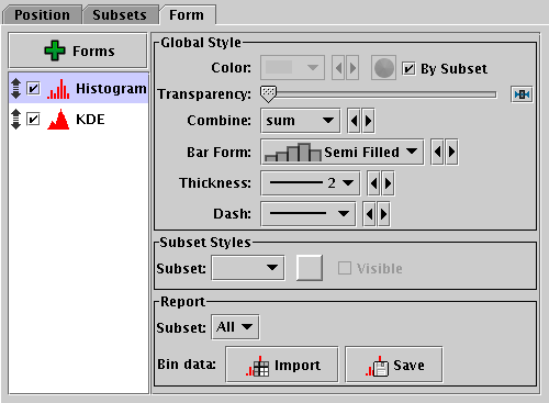
Form tab of Histogram layer control
The Form tab lets you define how the specified data set is plotted. The stack on the left gives a list of forms currently included in the plot, and the panel on the right shows the detailed configuration for the currently selected form.
When first added, the stack contains a single entry,
Histogram, which plots a simple histogram.
The colour is by default determined by the setting in the
Subsets tab.
This may be all you need, but if you want to use other histogram-like
plots such as Kernel Density Estimates, you can add new forms to the stack
using items in the popup menu from the Forms button
above the stack.
You can remove a form by selecting it and using the
Remove () item in the same menu.
You can also activate/deactivate entries in the stack with the checkbox
and move them up and down with the drag handle as usual.
The available forms are currently
 Histogram; some variants on the idea of a Kernel Density Estimate:
 KDE,
KDE,  KNN,
KNN,  Densogram;
and
Densogram;
and  Gaussian, which effectively plots a Gaussian best fit
to a histogram.
Gaussian, which effectively plots a Gaussian best fit
to a histogram.
The Global Style and Subset Style sub-panels control shared and per-subset configuration specific to the selected form as described in Appendix A.4.2.2.
Histograms have some additional configuration items,
as described in the
Bins ( )
fixed control.
When a histogram layer control is used in the
Histogram window,
those configuration items are found in the
Bins fixed control, where they control the settings
for all the histogram layers in the plot.
However, if you use a histogram layer in a
Plane plot,
those items will appear as additional items in the Form tab
and can be controlled separately for each histogram.
)
fixed control.
When a histogram layer control is used in the
Histogram window,
those configuration items are found in the
Bins fixed control, where they control the settings
for all the histogram layers in the plot.
However, if you use a histogram layer in a
Plane plot,
those items will appear as additional items in the Form tab
and can be controlled separately for each histogram.
The Area layer control ( )
allows you to plot a two-dimensional shape from each row of a table.
This might typically be something like an instrument coverage footprint
corresponding to an observation.
The shape may be specified in various different ways:
as an STC-S region specification string
(as found for instance in the
)
allows you to plot a two-dimensional shape from each row of a table.
This might typically be something like an instrument coverage footprint
corresponding to an observation.
The shape may be specified in various different ways:
as an STC-S region specification string
(as found for instance in the s_region column of
ObsCore or EPN-TAP query results),
as an array specification of polygons or circles,
or as an ASCII-encoded MOC.
You can add one of these controls to the stack by using the
Add Area Control ( ) button
in the control panel toolbar
or the corresponding item in the Layers menu
for suitable plot types
(Plane,
Sky or
Sphere).
) button
in the control panel toolbar
or the corresponding item in the Layers menu
for suitable plot types
(Plane,
Sky or
Sphere).
Areas specified in this way are generally intended for displaying relatively small shapes such as instrument footprints. Larger areas may also be specified, but there may be issues with use, for instance auto-determination of the initial plot region may not work so well, and the rendering of shapes that are large relative to the sky may be inaccurate. These issues may be addressed in future releases.
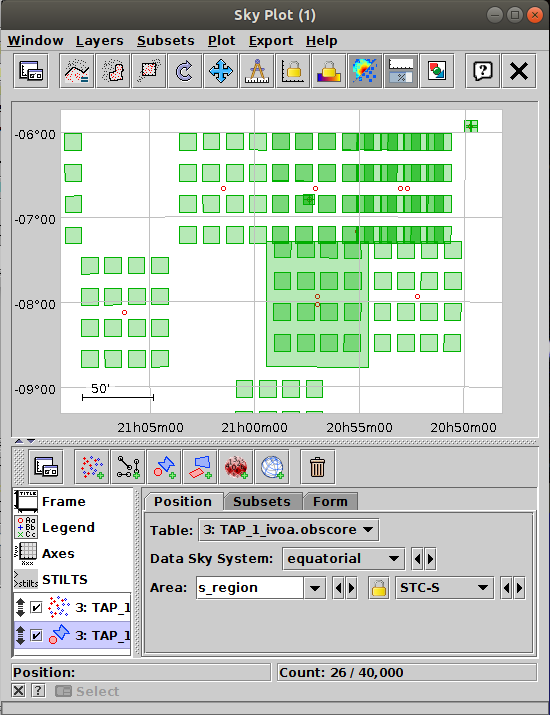
Sky Plot Window with an Area control
This control is a Table Data control as described in Appendix A.4.2.2. That section explains the Subsets tab; the Position and Form tabs are described in more detail below.
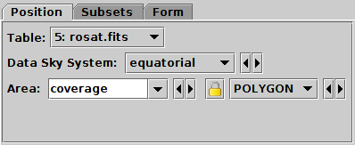
Position tab of Area layer control, for Sky Plot
In the Position tab, you just need to
select the input table using the Table selector,
and then supply the expression for the region specification
in the Area selector.
This area value will typically be a table column containing the relevant
information, for instance the s_region column
in tables resulting from an ObsCore or EPN-TAP query.
However, it's also possible to enter a suitable expression,
for instance "array(RA,DEC,RADIUS)" if you want
to specify a CIRCLE-format shape given position and radius
columns in the table.
The area may be specified in various formats, currently:
<frame>, <refpos> and
<flavor> metadata are ignored,
polygon winding direction is ignored (small polygons are assumed)
and the INTERSECTION and NOT
constructions are not supported.
The non-standard MOC construction is supported.
 ) button to stop it happening.
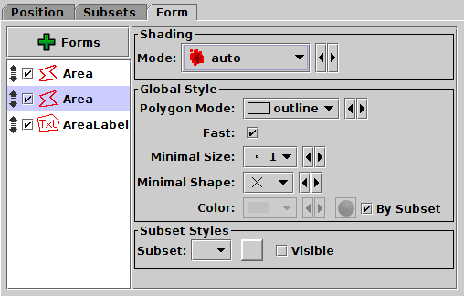
Form tab of Area layer control
The Form tab lets you define how the specified region data will be plotted. The list on the left gives a list of forms currently being plotted, and the panel on the right shows the detailed configuration for the currently selected form.
The following forms are currently available for the Area plot:
 Area:
draws an outlined or filled area
Area:
draws an outlined or filled area Central:
plots the central point of an area
Central:
plots the central point of an area AreaLabel:
adds a text label near the center of an area
AreaLabel:
adds a text label near the center of an areaYou can add a new form using the Forms button.
Each such form can be configured separately using a panel
divided into two parts:
The Spectrogram Layer Control ( )
plots a spectrum at successive (usually, but not necessarily,
regularly-spaced) points in a time series.
It is only available for the
Time Plot Window;
you can add one of these controls to the stack by using the
Add Spectrogram Control (
)
plots a spectrum at successive (usually, but not necessarily,
regularly-spaced) points in a time series.
It is only available for the
Time Plot Window;
you can add one of these controls to the stack by using the
Add Spectrogram Control ( ) button
in the control panel toolbar,
or the corresponding item in the Layers menu.
) button
in the control panel toolbar,
or the corresponding item in the Layers menu.
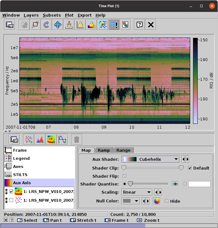
Time Plot window with a Spectrogram layer
This control has layer-specific tabs Data and Style, described below. The Zone tab is described in Appendix A.4.14.1.
To control the colour map used to represent the spectral values,
use the Aux fixed control.
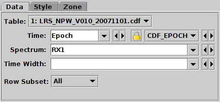
Spectrogram control Data tab
The Data tab allows you to specify which values from a table will generate a spectrogram. It has the following fields:
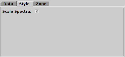
Spectrogram control Style tab
The Style tab configures the plotting style. Options are:
If this option is unchecked, or if no suitable array can be found, the vertical axis just represents channel indices and so is labelled from 0 to the number of channels per spectrum.
This configuration item is somewhat experimental; the details of how the spectral axis is configured may change in future releases.
The XYArray layer control ( )
can be used to plot points, lines and error bars,
but unlike the Position Layer Control
it works with table cells whose values are arrays giving multiple coordinates,
rather than single values.
It is typically used where the value stored in each cell of a column
is an array representing a whole spectrum or time series,
or some related quantity (such as errors, frequencies, epochs etc).
Each row of the table therefore corresponds to a full spectrum,
timeseries, or other array of coordinate pairs.
)
can be used to plot points, lines and error bars,
but unlike the Position Layer Control
it works with table cells whose values are arrays giving multiple coordinates,
rather than single values.
It is typically used where the value stored in each cell of a column
is an array representing a whole spectrum or time series,
or some related quantity (such as errors, frequencies, epochs etc).
Each row of the table therefore corresponds to a full spectrum,
timeseries, or other array of coordinate pairs.
You can add one of these controls to the Plane plot stack by using the
Add XYArray Control ( ) button
in the control panel toolbar,
or the corresponding item in the Layers menu.
You may need to deactivate the default
Position Layer Control stack entry () as well
to avoid confusion and make sure the ranging works correctly.
This control is only available for the
Plane plot.
) button
in the control panel toolbar,
or the corresponding item in the Layers menu.
You may need to deactivate the default
Position Layer Control stack entry () as well
to avoid confusion and make sure the ranging works correctly.
This control is only available for the
Plane plot.
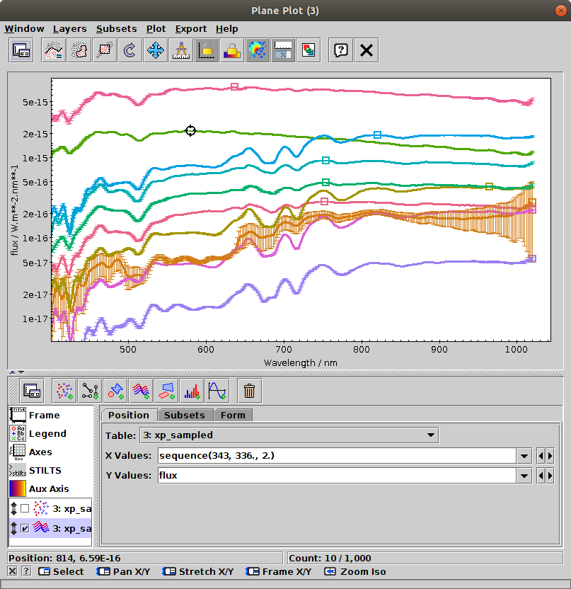
Plane Plot window with an XYArray layer
Note that unlike for instance plots of simple X,Y positions,
there is no obvious single position associated with each plotted row
(X/Y array pair, or wiggly line).
That means that by default, you can't click on a plotted line to
activate it,
or see it highlighted when you activate the corresponding row by
clicking on it in the Data Window.
To do that, you can use the
Handles Form ( ),
which plots a "handle" marker at some configurable
reference position near each line.
That then serves as the effective position on the plot for each row
for the purposes of activation, highlighting, graphical subset definition, etc.
For convenience, a disabled Handles entry is added by default to the
stack in the Forms tab,
so you can enable it just by clicking on its checkbox.
The handle positions and appearance can be adjusted using
the configuration panel.
),
which plots a "handle" marker at some configurable
reference position near each line.
That then serves as the effective position on the plot for each row
for the purposes of activation, highlighting, graphical subset definition, etc.
For convenience, a disabled Handles entry is added by default to the
stack in the Forms tab,
so you can enable it just by clicking on its checkbox.
The handle positions and appearance can be adjusted using
the configuration panel.
This control is a Table Data control as described in Appendix A.4.2.2. That section explains the Subsets tab; the Position and Form tabs are described in more detail below.
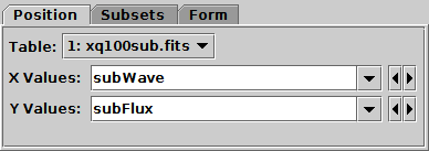
Position tab of XYArray layer control
In the Position tab you have to fill in
array values for the X Values and Y Values
plot coordinates.
The contents can be array-valued column names or expressions.
For each row, the X and Y coordinates must be arrays of the same length
(if they are not, nothing will be plotted for that row),
though different rows may have different array lengths.
To manipulate array values, some of the expression language functions
in the Arrays class may be useful;
for instance the expression "multiply(flux,1./mean(flux))"
can be used to normalise an input flux array.
For most of the available plots, if either the X or Y array value is missing,
it will be interpreted as a sequence (0,1,2,...) of the same length
as the array that is present.
TOPCAT will try to fill in the X and Y coordinates with suitable
array values from the table, if it can find some.
As well as array-valued columns, array-valued table parameters
can be used, and are often suitable for the X axis;
these can be referred to using the syntax "param$<name>",
as explained in Section 7.3.
It helps if columns are declared with fixed array sizes, where applicable.
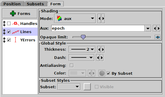
Form tab of XYArray layer control
The Form tab lets you define how the specified data set is plotted. The list on the left gives a list of forms currently being plotted, and the panel on the right shows the detailed configuration for the currently selected form.
The available forms for an XYArray plot
(select them using the Forms button)
are currently
 Lines:
draws a line between the X,Y positions Marks:
draws a marker for each X,Y position Handles:
draws a single marker at a reference position for
the whole array of X,Y pairs
Lines:
draws a line between the X,Y positions Marks:
draws a marker for each X,Y position Handles:
draws a single marker at a reference position for
the whole array of X,Y pairs YErrors:
draws a vertical error bar at each X,Y position
YErrors:
draws a vertical error bar at each X,Y position XYErrors:
draws horizontal and/or vertical error bars at each X,Y position
XYErrors:
draws horizontal and/or vertical error bars at each X,Y position StatLine:
draws a single line giving per-element combinations (e.g. mean)
of the input array values
StatLine:
draws a single line giving per-element combinations (e.g. mean)
of the input array values StatMark:
draws a marker for each per-element combination (e.g. mean)
of the input array values
StatMark:
draws a marker for each per-element combination (e.g. mean)
of the input array values ArrayQuantile:
draws quantile ranges for samples from the input array values
ArrayQuantile:
draws quantile ranges for samples from the input array valuesThe Function layer control ( )
is only available for the
Plane,
Histogram and
Time plots.
You can add one of these controls to the stack by using the
Add Function Control (
)
is only available for the
Plane,
Histogram and
Time plots.
You can add one of these controls to the stack by using the
Add Function Control ( ) button
in the control panel toolbar,
or the corresponding item in the Layers menu.
) button
in the control panel toolbar,
or the corresponding item in the Layers menu.
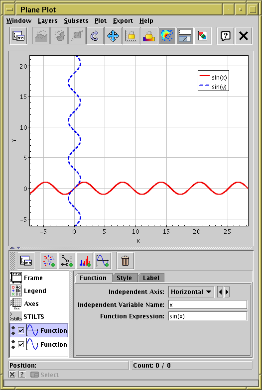
Plane plot with two function layers plotted, one as a function of Horizontal axis value, and one as a function of Vertical axis value
This control has three tabs, Function, Style and Label, described below.
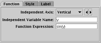
Function control Function tab
The Function tab defines the function to be plotted and has the following fields:
x for a horizontal independent variable
and y for a vertical independent variable,
but any string that is a legal expression language identifier
(starts with a letter, continues with letters, numbers, underscores)
can be used.
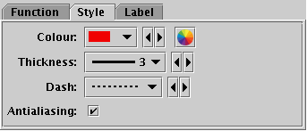
Function control Style tab
The Style tab configures the plotting style. Options are:
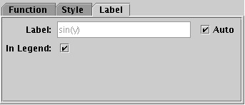
Function control Label tab
The Label tab allows you to choose the text that appears in the legend. Options are:
The SkyGrid layer control ( )
is available from the Sky Plot Window,
and plots an additional axis grid on the celestial sphere.
This can be overlaid on the default sky axis grid
so that axes for multiple sky coordinate systems
are simultaneously visible.
You can add one of these controls to the SkyPlot stack by using the
Add SkyGrid Control (
)
is available from the Sky Plot Window,
and plots an additional axis grid on the celestial sphere.
This can be overlaid on the default sky axis grid
so that axes for multiple sky coordinate systems
are simultaneously visible.
You can add one of these controls to the SkyPlot stack by using the
Add SkyGrid Control ( ) button
in the control panel toolbar,
or the corresponding item in the Layers menu.
) button
in the control panel toolbar,
or the corresponding item in the Layers menu.
Note that some of the configuration items for this plot layer, such as grid line antialiasing and the decimal/sexagesimal flag, are inherited from the values set for the main sky plot grid in the Sky Axes Control.
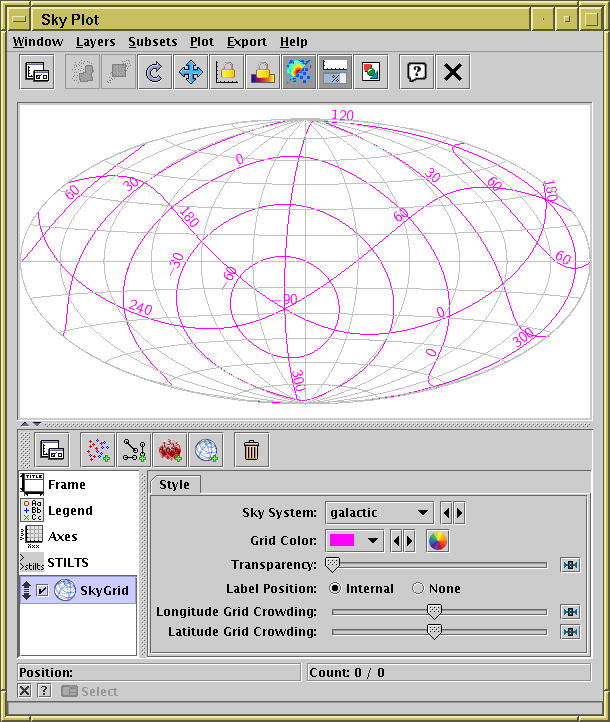
Sky plot with no data, but an additional Galactic sky axis grid plotted over the default equatorial grid.
This control has only one tab, Style, with the following fields:
The SphereGrid layer control ()
plots a spherical net centered on the coordinate origin.
It is available from the
Sphere and
Cube plot windows,
and you can add one of these controls to the stack by using the
Add SphereGrid Control () button
in the control panel toolbar,
or the corresponding item in the Layers menu.
The plotted grid is currently not labelled, but it can provide orientation to make clear for instance the position of a bounding unit sphere. Its radius can be controlled by a slider or by entering a fixed value. Since the sphere is always centered on the origin, if the whole visible cube is far from the origin, it may be that few or none of the grid lines show up on the plot.
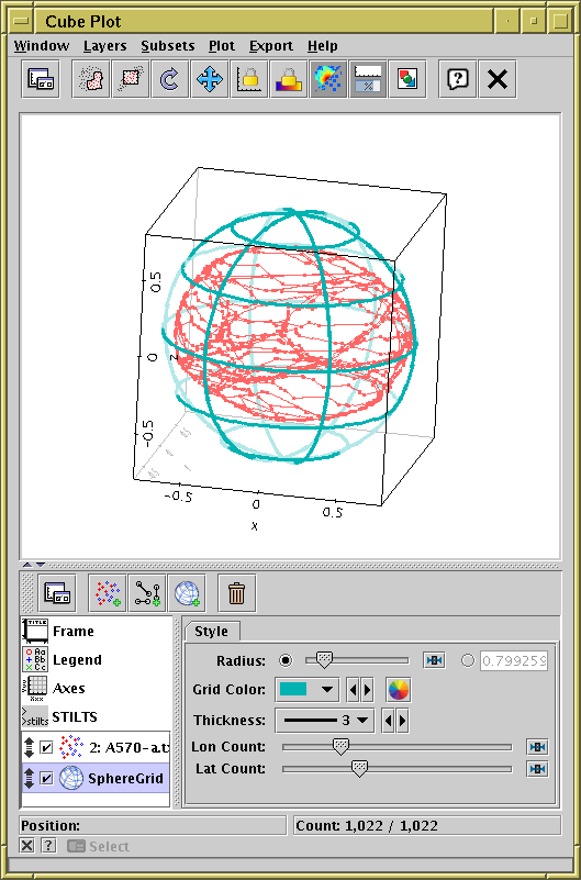
Plot of the XYZ vertices providing surface of an asteroid (48 Doris) with a spherical grid overplotted.
This control has only one tab, Style, with the following fields:
Plot "forms" are the instructions for what shapes to actually paint on the plotting surface given some positional data from a table. The most obvious (Mark) is simply to plot a marker with a fixed size and shape at each data position. However, there is a range of other things you might want to do, including error bars, vectors, contours, text labels, ...
The options provided are described, with the additional configuration information required, in the following sections. Not all are available for every plot type.
The Mark form ()
simply plots markers with a fixed shape and size.
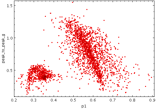
Example Mark plot
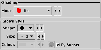
Mark form configuration panel
Configuration options are:
The Size form ( )
plots markers of a fixed shape
whose size varies according to a supplied data coordinate.
The marker size thus represents an additional dimension of the plot.
)
plots markers of a fixed shape
whose size varies according to a supplied data coordinate.
The marker size thus represents an additional dimension of the plot.
The actual size of the markers depends on the setting of the Auto Scale option. If autoscaling is off, then the basic size of each marker is the input data value in units of pixels. If autoscaling is on, then the data values are gathered for all the currently visible points, and a scaling factor is applied so that the largest ones will be a sensible size (a few tens of pixels). This basic size can be further adjusted with the Scale slider.
Currently data values of zero always correspond to marker size of zero, negative data values are not represented, and the mapping is linear. An absolute maximum size on markers is also imposed. Other options may be introduced in future.
Note the scaling to size is in terms of screen dimensions (pixels). For sizes that correspond to actual data values, the Error form may be more appropriate.
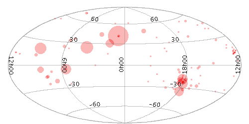
Example Size plot
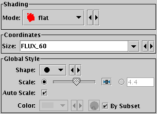
Size form configuration panel
The configuration options are:
If auto-scaling is off, then markers will keep exactly the same screen size during pan and zoom operations; if it's on, then the visible sizes will change according to what other points are currently plotted.
The SizeXY form ( )
plots a shaped marker whose width and height vary independently
acoording to two supplied data coordinates.
The marker shape can thus encode two additional dimensions of the plot.
)
plots a shaped marker whose width and height vary independently
acoording to two supplied data coordinates.
The marker shape can thus encode two additional dimensions of the plot.
The actual size of the markers depends on the setting of the Auto Scale option. If autoscaling is off, the basic dimensions of each marker are given by the input data values in units of pixels. If autoscaling is on, the data values are gathered for all the currently visible points, and scaling factors are applied so that the largest ones will be a sensible size (a few tens of pixels). This autoscaling happens independently for the X and Y directions. The basic sizes can be further adjusted with the Scale slider.
Currently data values of zero always correspond to marker extent of zero, negative data values are not represented, and the mapping is linear. An absolute maximum size on markers is also imposed. Other options may be introduced in future.
Note the scaling to size is in terms of screen dimensions (pixels). For sizes that correspond to actual data values, the Error form may be more appropriate.
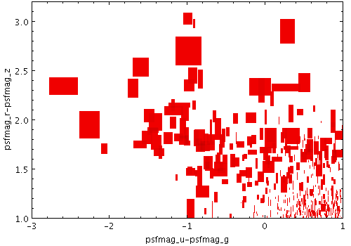
Example SizeXY plot
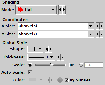
SizeXY form configuration panel
The configuration options are:
If auto-scaling is off, then markers will keep exactly the same screen size during pan and zoom operations; if it's on, then the visible sizes will change according to what other points are currently plotted.
The Vector form ( )
plots directed lines from the
data position given delta values for the coordinates.
The plotted markers are typically little arrows, but there are
other options.
)
plots directed lines from the
data position given delta values for the coordinates.
The plotted markers are typically little arrows, but there are
other options.
In some cases such delta values may be the actual magnitude required for the plot, but often the vector data represents a value which has a different magnitude or is in different units to the positional data. As a convenience for this case, the plotter can optionally scale the magnitudes of all the vectors to make them a sensible size (so the largest ones are a few tens of pixels long). This scaling can be adjusted or turned off using the Scale and Auto Scale options below.
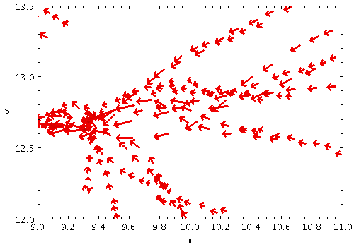
Example XYVector plot
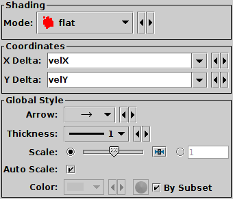
Vector form configuration panel
The configuration options are:
The SkyVector form ()
plots directed lines from the data position
given relative offsets to longitude.cos(latitude) and latitude
on the celestial sphere.
The plotted markers are typically little arrows, but there are
other options.
In some cases such delta values may be the actual magnitude required for the plot, but often the vector data represents a value which has a different magnitude or is in different units to the positional data (for instance proper motions). As a convenience for this case, the plotter can optionally scale the magnitudes of all the vectors to make them a sensible size (so the largest ones are a few tens of pixels long). This scaling can be adjusted or turned off using the Scale and Auto Scale options below.
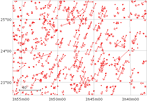
Example SkyVector plot
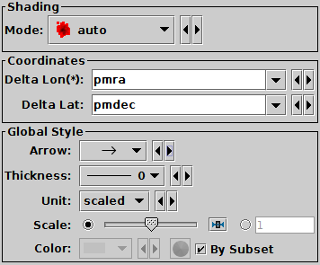
SkyVector form configuration panel
The configuration options are:
The Error Bars form ()
draws symmetric or asymmetric
error bars in some or all of the dimensions of a 1-, 2- or 3-dimensional
Cartesian plot.
The shape of the error "bars" is quite configurable, including
(for 2- and 3-d errors) ellipses, rectangles etc, aligned with the axes
(for rotated ellipses and rectangles,
see the XYEllipse and
XYCorr forms).
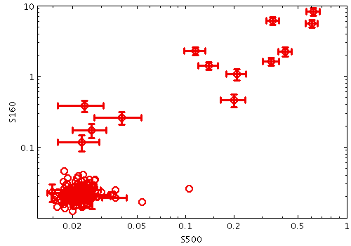
Example XYError plot
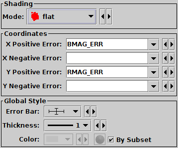
Error Bars form configuration panel
The configuration options are:
0" for the corresponding negative error.
The XYEllipse form ( )
plots an ellipse (or rectangle, triangle, or other similar figure)
defined by two principal radii and an optional angle of rotation,
the so-called position angle.
This angle, if specified, is in degrees and gives the angle
counterclockwise from the horizontal axis to the first principal radius.
)
plots an ellipse (or rectangle, triangle, or other similar figure)
defined by two principal radii and an optional angle of rotation,
the so-called position angle.
This angle, if specified, is in degrees and gives the angle
counterclockwise from the horizontal axis to the first principal radius.
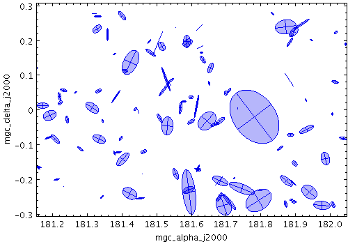
Example XYEllipse plot
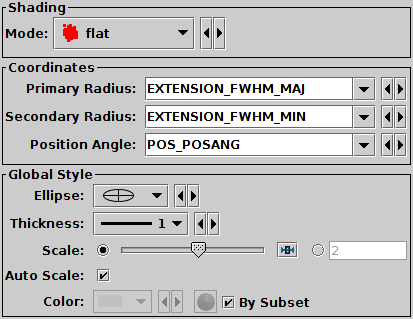
XYEllipse form configuration panel
The configuration options are:
The SkyEllipse ( ) form
plots an ellipse (or rectangle, triangle, or other similar figure)
defined by two principal radii and an optional angle of rotation,
the so-called position angle.
This angle, if specified, is in degrees and gives the angle
from the North pole towards the direction of increasing longitude
on the longitude axis.
) form
plots an ellipse (or rectangle, triangle, or other similar figure)
defined by two principal radii and an optional angle of rotation,
the so-called position angle.
This angle, if specified, is in degrees and gives the angle
from the North pole towards the direction of increasing longitude
on the longitude axis.
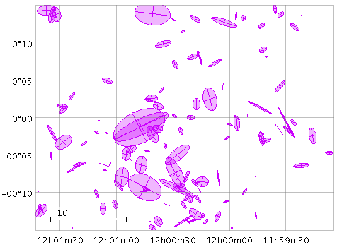
Example SkyEllipse plot
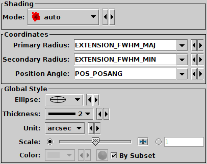
SkyEllipse form configuration panel
The configuration options are:
The XYCorr ( ) form
plots an error ellipse (or rectangle or other similar figure)
defined by errors in the X and Y directions,
and a correlation between the two errors.
) form
plots an error ellipse (or rectangle or other similar figure)
defined by errors in the X and Y directions,
and a correlation between the two errors.
The supplied correlation is a dimensionless value in the range -1..+1 and is equal to the covariance divided by the product of the X and Y errors. The covariance matrix is thus:
   [  xerr*xerr         xerr*yerr*xycorr  ]
   [  xerr*yerr*xycorr  yerr*yerr         ]
This plot type is suitable for use with the
<x>_error and
<x>_<y>_corr
columns in the Gaia source catalogue.
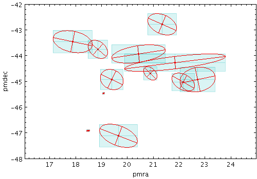
Example XYCorr plot
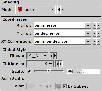
XYCorr form configuration panel
The configuration options are:
x_y_corr values
supplied in the Gaia source catalogue.
The SkyCorr () form
plots an error ellipse (or rectangle or other similar figure)
on the sky defined by errors in the longitude and latitude directions,
and a correlation between the two errors.
The error in longitude is considered to be premultiplied by the cosine of the latitude, i.e. both errors correspond to angular distances along a great circle.
The supplied correlation is a dimensionless value in the range -1..+1 and is equal to the covariance divided by the product of the lon and lat errors. The covariance matrix is thus:
   [  lonerr*lonerr       lonerr*laterr*corr  ]
   [  lonerr*laterr*corr  laterr*laterr       ]
This plot type is suitable for use with the
ra_error, dec_error and ra_dec_corr
columns in the Gaia source catalogue.
Note however that Gaia positional errors are generally quoted
in milli-arseconds (mas),
while this plotter requires lon/lat errors in degrees,
so to plot true error ellipses
it is necessary to divide the Gaia error values by 3.6e6.
In most plots, Gaia position errors are much too tiny to see!
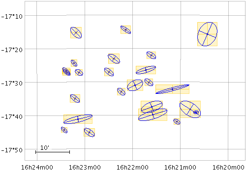
Example SkyCorr plot
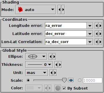
SkyCorr form configuration panel
The configuration options are:
ra_dec_corr value
supplied in the Gaia source catalogue.
The Polygon ( ) form
plots filled or outlined polygons with an arbitrary number of vertices.
The first vertex is given in the
Position Layer Control's
Position tab,
and the others are given in the Coordinates box within the
Form tab.
) form
plots filled or outlined polygons with an arbitrary number of vertices.
The first vertex is given in the
Position Layer Control's
Position tab,
and the others are given in the Coordinates box within the
Form tab.
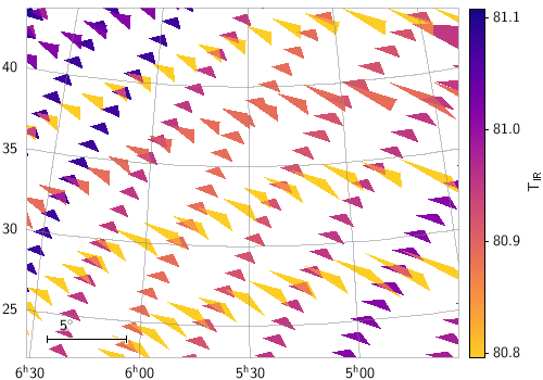
Example Polygon plot
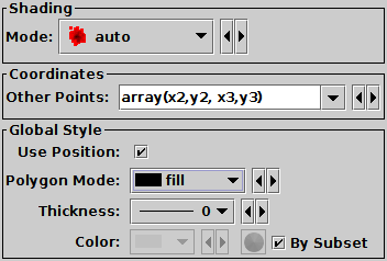
Polygon form configuration panel
The configuration options are:
(x2,y2, x3,y3, x4,y4).
Expression language functions including
array(a,b,c,...)
from the Arrays class, and
parseDoubles(txt)
from the Conversions class,
can be useful here.
Although the first coordinate pair is supposed to be given in the
Position tab and not in this array, if it's more convenient to
repeat the first pair here it doesn't usually affect the plot's
appearance.
outline:
draws a line round the outside of the polygonfill:
fills the interior of the polygoncross:
draws a line round the outside of the polygon
and lines between all the verticesThe Line form ()
draws a point-to-point line joining
up the points making up the data set.
There are additional options to pre-sort the points according
to their order on the X or Y axis
(using the Sort Axis control),
and to vary the colour of the line along its length
(using the Aux coordinate).
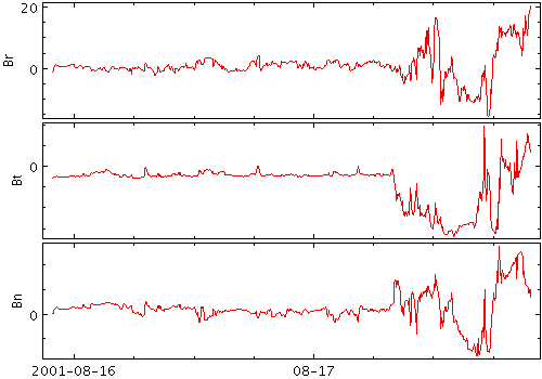
Example Line plot
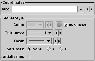
Line form configuration panel
The configuration options are:
The Line3d form ()
draws a point-to-point line joining
up the positions of the points in three dimensions.
There are additional options to pre-sort the points
by a given quantity before drawing the lines,
and to colour the line along its length using an auxiliary coordinate.
Note that the line positioning in 3d and the line segment aux colouring is somewhat approximate. In most cases it is good enough for visual inspection, but pixel-level examination may reveal discrepancies.
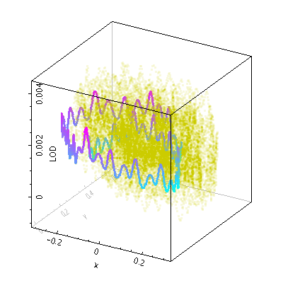
Example Line3d plot
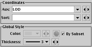
Line3d form configuration panel
The configuration options are:
The Linear Fit form ( )
determines a least-squares best fit of a line to the data points,
optionally weighted by a given value, and plots the corresponding line.
)
determines a least-squares best fit of a line to the data points,
optionally weighted by a given value, and plots the corresponding line.
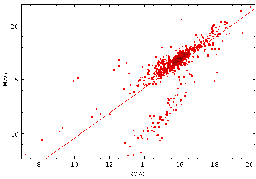
Example LinearFit plot
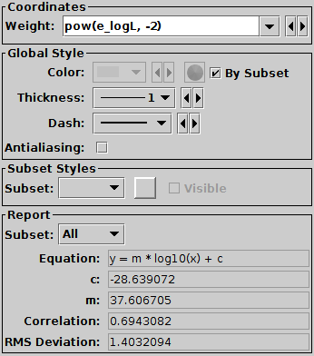
Linear Fit configuration panel
The configuration options are:
E are available for each point,
a suitable value for this may be 1./(E*E)
(equivalently pow(E,-2)).
As well as drawing the line onto the plot, the calculated fitting coefficients are displayed at the bottom of the form configuration panel, under the heading Report. Note the coefficients are calculated by subset, and are only displayed for one subset at a time. To see the calculated values, select the subset of interest in the Subset selector. The reported items are:
y=m*x+c,
but if one or both of the axes are plotted logarithmically,
the fit is performed to take account of this, and the equation
is displayed accordingly.
The Quantile form ()
plots a line through a given quantile of the values binned within
each pixel column (or row) of a plot.
The line is optionally smoothed using a configurable kernel and width,
to even out noise from the pixel binning.
Instead of a simple line through a given quantile, it is also
possible to fill the region between two quantiles.
One way to use this is to draw a line estimating a function y=f(x) (or x=g(y)) sampled by a noisy set of data points in two dimensions.
Note: In the current implementation, depending on the details of the configuration and the data, there may be some distortions or missing graphics near the edges of the plot. This may be improved in future releases, depending on feedback.
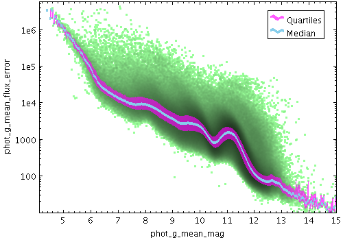
Example Quantile plot
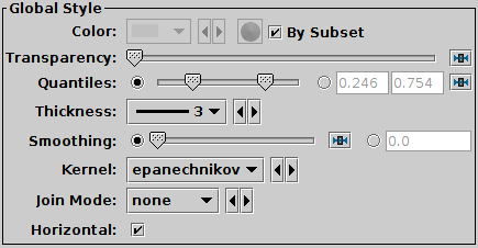
Quantile configuration panel
The configuration options are:
The radio buttons let you toggle between using the slider to set the quantile value(s) or entering them in the text fields. If the two values are identical, you can leave the second text field blank.
You can adjust it using the slider (wider smoothing to the right) or enter a value in data coordinates explicitly in the text field. If the smoothed axis is logarithmic, the value is a multiplication factor rather than an additive increment.
The available options are:
The available options are:
The Label form ( )
draws a text label by each point position.
)
draws a text label by each point position.
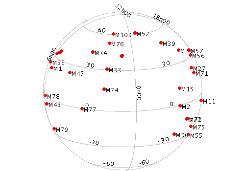
Example Label plot
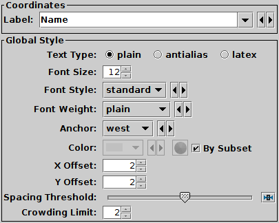
Label form configuration panel
The configuration options are:
The Contour form ( )
plots position density contours.
These provide another way
(alongside the Auto,
Density and
Weighted shading modes)
to visualise the characteristics of overdense regions in a crowded plot.
)
plots position density contours.
These provide another way
(alongside the Auto,
Density and
Weighted shading modes)
to visualise the characteristics of overdense regions in a crowded plot.
The contours are currently drawn as pixels rather than lines, so they don't look very beautiful in exported vector output formats (PDF, SVG, PostScript).
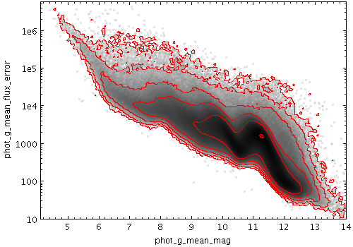
Example Contour plot

Contour form configuration panel
The configuration options are:
mean which traces the
mean values of a quantity and
sum which traces the
weighted sum.
Other values such as
median
are of dubious validity because of the way that the
smoothing is done.
This value is ignored if the weighting coordinate Weight is not set.
The available options are:
sum: the sum of all the combined values per binmean: the mean of the combined valuesmedian:
the median of the combined values (may be slow)stdev:
the sample standard deviation of the combined valuesmin: the minimum of all the combined valuesmax: the maximum of all the combined valuescount:
the number of non-blank values per bin (weight is ignored)The Grid form ( )
plots 2-d point data aggregated into rectangular cells on the plotting plane.
You can optionally use a weighting for the points,
and you can configure how the values are combined to produce the
output pixel values (colours).
You can use this layer type in various ways,
including as a 2-d histogram or weighted density map,
or to plot gridded data.
)
plots 2-d point data aggregated into rectangular cells on the plotting plane.
You can optionally use a weighting for the points,
and you can configure how the values are combined to produce the
output pixel values (colours).
You can use this layer type in various ways,
including as a 2-d histogram or weighted density map,
or to plot gridded data.
The X and Y dimensions of the grid cells (or equivalently histogram bins) can be configured in terms of either the data coordinates or relative to the plot dimensions.
The shading is done using the shared colour map. This colour map is used by all currently visible Grid, Aux and Weighted layers. When at least one such layer is being plotted, the Aux Axis control is visible in the control panel, which allows you to configure the colour map, range, ramp display etc.
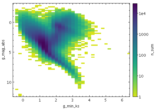
Example Grid plot
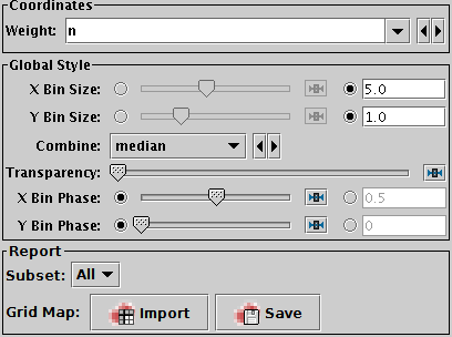
Grid form configuration panel
The configuration options are:
sum) but not others (e.g. mean).
count or sum.
However, if there is a non-blank Weight coordinate,
one of the other values such as mean may be more revealing.
The following options (some are more useful than others) are currently available:
sum: the sum of all weightssum-per-unit:
the sum of all weights per unit of bin sizemean: the mean of all weightsmedian: the median of all weights (can be slow)q1: the first quartile of all weights (can be slow)q3: the third quartile of all weights (can be slow)min: the minimum weightmax: the maximum weightstdev: the sample standard deviation of all weightscount: the number of points plotted
(weight value is ignored, this is like Density mode)count-per-unit:
the number of points plotted per unit of bin size
(weight value is ignored)hit: one if any point is plotted, blank otherwise
(weight value is ignored, this is like Flat mode)The Report panel provides information calculated by the plot:
 ) option
loads the data as a new table in the TOPCAT application, and
the Save (
) option
loads the data as a new table in the TOPCAT application, and
the Save ( ) option
lets you save it directly to disk in one of the available table formats.
This information is also available from the Export menu.
) option
lets you save it directly to disk in one of the available table formats.
This information is also available from the Export menu.
The SkyDensity form ( )
plots a density map on the sky using a HEALPix grid
with a configurable resolution.
You can optionally use a weighting for the data values to accumulate
within each HEALPix tile,
and you can configure how the weighted values are combined to
generate the eventual pixel values (and hence colours).
HEALPix
is a tiling scheme for the sky which uses square-ish pixels
of equal area to cover the celestial sphere.
)
plots a density map on the sky using a HEALPix grid
with a configurable resolution.
You can optionally use a weighting for the data values to accumulate
within each HEALPix tile,
and you can configure how the weighted values are combined to
generate the eventual pixel values (and hence colours).
HEALPix
is a tiling scheme for the sky which uses square-ish pixels
of equal area to cover the celestial sphere.
The shading is done using the shared colour map. This colour map is used by all currently visible SkyDensity, Grid, Aux and Weighted layers. When at least one such layer is being plotted, the Aux Axis control is visible in the control panel, which allows you to configure the colour map, range, ramp display etc.
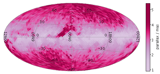
Example SkyDensity plot
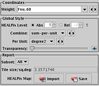
SkyDensity form configuration panel
The configuration options are:
For density-like values
(count-per-unit, sum-per-unit)
the scaling is additionally influenced by the
Per Unit option.
The following options (some are more useful than others) are currently available:
sum:
the sum of all the combined values per binsum-per-unit:
the sum of all the combined values per unit of bin sizecount:
the number of non-blank values per bin (weight is ignored)count-per-unit:
the number of non-blank values per unit of bin size
(weight is ignored)mean:
the mean of the combined valuesmedian:
the median of the combined values (may be slow)q1:
the first quartile of the combined values (may be slow)q3:
the third quartile of the combined values (may be slow)min: the minimum of all the combined valuesmax: the maximum of all the combined valuesstdev:
the sample standard deviation of the combined valueshit:
1 if any values present, NaN otherwise (weight is ignored)count-per-unit or sum-per-unit).
If the Combination mode is calculating values per unit area,
this configures the area scale in question.
For non-density-like combination modes
(e.g. sum or mean)
it has no effect.
The available options are:
steradian: steradiandegree2: square degreearcmin2: square arcminutearcsec2: square arcsecondmas2: square milliarcsecuas2: square microarcsecThe Report panel provides information calculated by the plot:
 ) option
loads the data as a new table in the TOPCAT application, and
the Save (
) option
loads the data as a new table in the TOPCAT application, and
the Save ( ) option
lets you save it directly to disk in one of the available table formats.
This information is also available from the Export menu.
) option
lets you save it directly to disk in one of the available table formats.
This information is also available from the Export menu.
Some notes apply for this export:
COORDSYS header) is determined by the current
value of the View Sky System, as reported in the
Sky Axes Control.The SkyVecField form ( )
plots a field of arrows on a HEALPix grid corresponding to the
aggregated (typically averaged) value of a 2-d vector quantity
such as proper motion for the points in each HEALPix cell.
)
plots a field of arrows on a HEALPix grid corresponding to the
aggregated (typically averaged) value of a 2-d vector quantity
such as proper motion for the points in each HEALPix cell.
Currently, the visible length of the vectors is dependent on the order of the grid; they are normalised to appear with a length comparable to the size of the HEALPix pixels. This length can be adjusted by use of the Scale control.
By default, the absolute values of the vectors are plotted. However, if the Relative option is set, the mean vector value averaged over the visible plot area will be calculated and subtracted from all the plotted vectors. The effect of this is to show local variations rather than absolute values of the vectors over the visible area. The value of such mean offsets is displayed in the Report panel at the bottom of the layer control panel.
This form may be used in the Sky plot window. The VecField form does the same thing for a Plane plot.
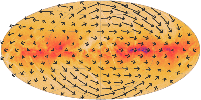
Example SkyVecField plot
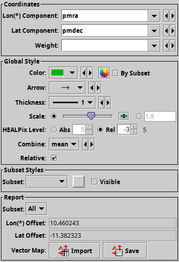
SkyVecField form configuration panel
The configuration options are:
The Report gives you access to the calculations made during plotting:
) option
loads the data as a new table in the TOPCAT application, and
the Save () option
lets you save it directly to disk in one of the available table formats.
These options are also available from the Export menu.
Some notes apply for this export:
COORDSYS header) is determined by the current
value of the View Sky System, as reported in the
Sky Axes Control.If a two-dimensional dataset represents a single-valued function,
the Fill form ( ) will fill the area underneath
the function's curve with a solid colour.
Parts of the surface which would only be partially covered
(because of rapid function variation within the width of a single pixel)
are represented using appropriate alpha-blending.
The filled area may alternatively be that above the curve
or (in some plot types) to its left or right.
) will fill the area underneath
the function's curve with a solid colour.
Parts of the surface which would only be partially covered
(because of rapid function variation within the width of a single pixel)
are represented using appropriate alpha-blending.
The filled area may alternatively be that above the curve
or (in some plot types) to its left or right.
One example of its use is to reconstruct the appearance of a histogram plot from a set of histogram bins. For X,Y data which is not single-valued, the result may not be very useful.
This form may be used in the Plane or Time plot windows.
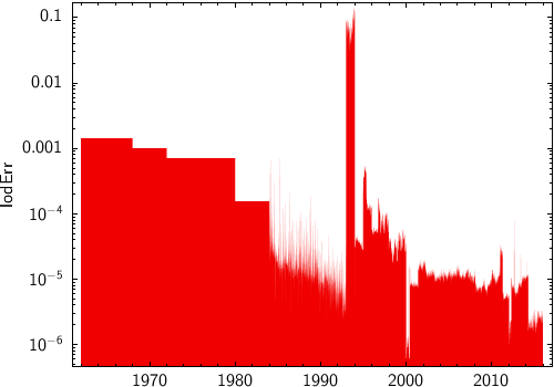
Example Fill plot
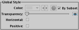
Fill form configuration panel
The configuration options are:
The VecField form ()
plots a field of arrows on a regular grid corresponding to the
aggregated (typically averaged) value of a 2-d vector quantity for the
points in each grid cell.
Currently, the X and Y components of the vectors are normalised separately and scaled so that the arrows are shown with components comparable to the dimensions of the grid cells. This length can be adjusted by use of the Scale control.
By default, the absolute values of the vectors are plotted. However, if the Relative option is set, the mean vector value averaged over the visible plot area will be calculated and subtracted from all the plotted vectors. The effect of this is to show local variations rather than absolute values of the vectors over the visible area. The value of such mean offsets is displayed in the Report panel at the bottom of the layer control panel.
The X and Y dimensions of the grid cells (or equivalently histogram bins) can be configured either in terms of the data coordinates or relative to the plot dimensions.
This form may be used in the Plane plot window. The SkyVecField form does the same thing for a Sky plot.
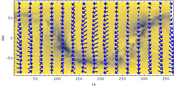
Example VecField plot
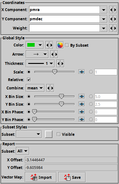
VecField form configuration panel
The configuration options are:
The Report gives you access to the calculations made during plotting:
) option
loads the data as a new table in the TOPCAT application, and
the Save () option
lets you save it directly to disk in one of the available table formats.
These options are also available from the Export menu.
The Histogram form ()
plots a histogram generated by binning samples along the X axis.
This form may be used in the Histogram, Plane or Time plot windows.
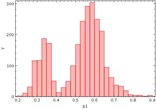
Example Histogram plot
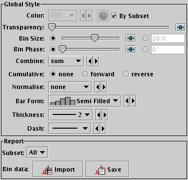
Histogram form configuration panel
These options always appear in the form configuration panel:
The available options are:
sum:
the sum of all the combined values per binsum-per-unit:
the sum of all the combined values per unit of bin sizecount:
the number of non-blank values per bin (weight is ignored)count-per-unit:
the number of non-blank values per unit of bin size
(weight is ignored)mean:
the mean of the combined valuesmedian:
the median of the combined values (may be slow)q1:
the first quartile of the combined values (may be slow)q3:
the third quartile of the combined values (may be slow)min: the minimum of all the combined valuesmax: the maximum of all the combined valuesstdev:
the sample standard deviation of the combined valueshit:
1 if any values present, NaN otherwise (weight is ignored))
for the Histogram window:
The Report panel gives you access to the bin values calculated by the plot:
 ) option
loads the data as a new table in the TOPCAT application, and
the Save (
) option
loads the data as a new table in the TOPCAT application, and
the Save ( ) option
lets you save it directly to disk in one of the available table formats.
This information is also available from the Export menu.
) option
lets you save it directly to disk in one of the available table formats.
This information is also available from the Export menu.
The KDE form ()
plots a discrete Kernel Density Estimate giving a smoothed
frequency of data values along the horizontal axis,
using a fixed-width smoothing kernel.
(for a variable-bandwidth kernel, see KNN).
This is a generalisation of a histogram in which the bins are always
1 pixel wide, and a smoothing kernel is applied to each bin. The width
and shape of the kernel may be varied.
This is suitable for cases where the division into discrete bins done by a normal histogram is unnecessary or troublesome.
Note this is not a true Kernel Density Estimate, since, for performance reasons, the smoothing is applied to the (pixel-width) bins rather than to each data sample. The deviation from a true KDE caused by this quantisation will be at the pixel level, hence in most cases not visually apparent.
This form may be used in the Histogram, Plane or Time plot windows.
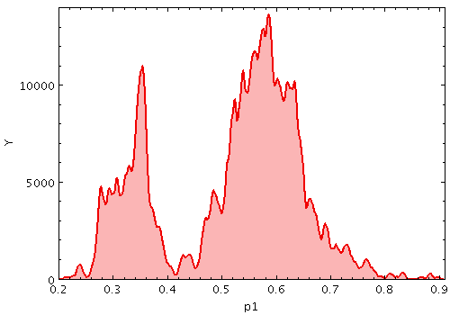
Example KDE plot
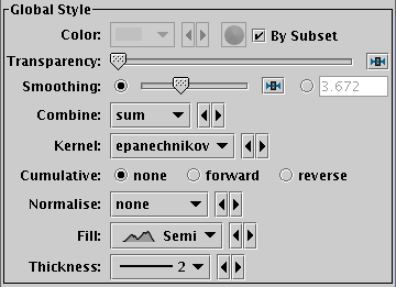
KDE form configuration panel
These options always appear in the form configuration panel:
sum-per-unit and
mean make sense,
others such as
sum do not.
The combined values are those given by the Weight coordinate, but if no weight is supplied, a weighting of unity is assumed.
The available options are:
sum:
the sum of all the combined values per binsum-per-unit:
the sum of all the combined values per unit of bin sizecount:
the number of non-blank values per bin (weight is ignored)count-per-unit:
the number of non-blank values per unit of bin size
(weight is ignored)mean:
the mean of the combined valuesmedian:
the median of the combined values (may be slow)q1:
the first quartile of the combined values (may be slow)q3:
the third quartile of the combined values (may be slow)min: the minimum of all the combined valuesmax: the maximum of all the combined valuesstdev:
the sample standard deviation of the combined valueshit:
1 if any values present, NaN otherwise (weight is ignored))
for the Histogram window:
Sliding the slider to the right makes the kernel width larger. The width in data units is shown in the text field on the right (if the X axis is logarithmic, this is a factor). Alternatively you can click the radio button near the text field, and enter the width in data units directly.
The available options are:
The KNN form ()
plots a discrete Kernel Density Estimate giving a smoothed
frequency of data values along the horizontal axis, using an adaptive
(K-Nearest-Neighbours) smoothing kernel. This is a generalisation of a
histogram in which the bins are always 1 pixel wide, and a
variable-bandwidth smoothing kernel is applied to each bin
(for a fixed-bandwidth kernel, see KDE).
The K-Nearest-Neighbour figure gives the number of points in each direction to determine the width of the smoothing kernel for smoothing each bin. Upper and lower limits for the kernel width are also supplied; if the upper and lower limits are equal, this is equivalent to a fixed-width kernel.
Note this is not a true Kernel Density Estimate, since, for performance reasons, the smoothing is applied to the (pixel-width) bins rather than to each data sample. The deviation from a true KDE caused by this quantisation will be at the pixel level, hence in most cases not visually apparent.
This form may be used in either the Histogram, Plane or Time plot windows.
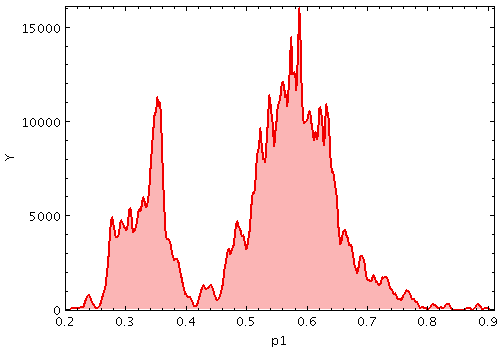
Example KNN plot
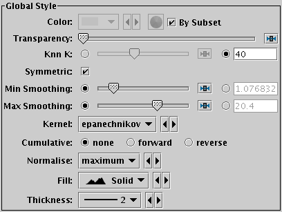
KNN form configuration panel
These options always appear in the form configuration panel:
You can either use the slider, or check the radio button on the right and enter the value in data units directly.
You can either use the slider, or check the radio button on the right and enter the value in data units directly.
)
for the Histogram window:
The available options are:
The Densogram form ()
represents smoothed density of data values along the horizontal axis using
a colourmap. This is like a Kernel Density Estimate (smoothed histogram
with bins 1 pixel wide), but instead of representing the data extent
vertically as bars or a line, values are represented by a fixed-size
pixel-width column of a colour from a colour map. A smoothing kernel,
whose width and shape may be varied, is applied to each data point.
This is a rather unconventional way to represent density data, and this plotting mode is probably not very useful. But hey, nobody's forcing you to use it.
This form may be used in either the Histogram, Plane or Time plot windows.
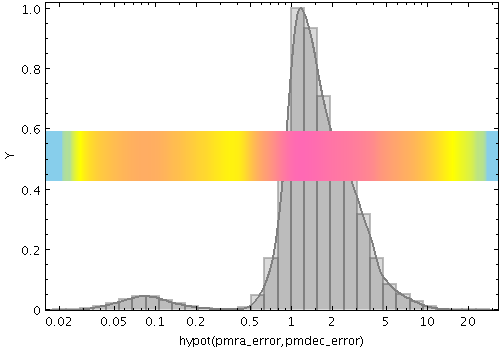
Example Densogram plot
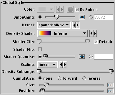
Densogram form configuration panel
These options always appear in the form configuration panel:
The default range is clipped at one end for colour maps that fade to white, so that all the plotted colours will be distinguishable against a white background. If you don't want that, you can uncheck Default and leave the handles at the extreme ends of the slider.
)
for the Histogram window:
Sliding the slider to the right makes the kernel width larger. The width in data units is shown in the text field on the right (if the X axis is logarithmic, this is a factor). Alternatively you can click the radio button near the text field, and enter the width in data units directly.
The available options are:
The Gaussian form ()
plots a best fit Gaussian to the histogram of a sample of data.
In fact, all it does is to calculate the mean and standard deviation
of the sample, and plot the corresponding Gaussian curve.
The mean and standard deviation values are reported by the plot
(see below).
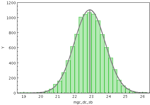
Example Gaussian plot
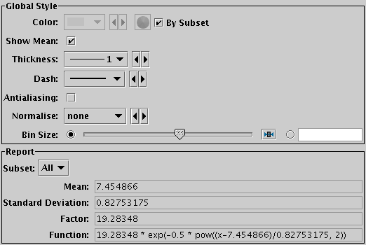
Gaussian fit configuration panel
These options always appear in the form configuration panel:
)
for the Histogram window:
As well as drawing the line onto the plot, the calculated fitting coefficients are displayed at the bottom of the form configuration panel, under the heading Report. Note the coefficients are calculated by subset, and are only displayed for one subset at a time. To see the calculated values, select the subset of interest in the Subset selector. The reported items are:
The Link2 form ()
is available from the
pair position layer control,
and plots a line linking the two points in a position pair.
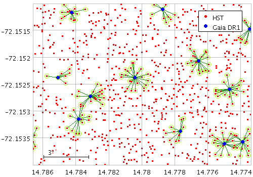
Example Link2 plot
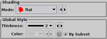
Link2 form configuration panel
Configuration options are:
The Mark2 () form
is available from the
pair position layer control,
and plots a marker of configurable
shape and size at both points in a position pair.
The same marker is used for both ends; if you want different points
you can use two single Mark forms.
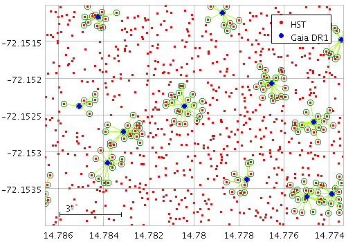
Example Mark2 plot
Mark2 form configuration panel
Configuration options are the same as for Mark:
The Poly4 () form
is available from the
quad position layer control,
and draws a quadrilateral defined by the coordinates of its vertices
supplied as 4 separate positions.
Various options for how it is drawn, such as filled or outlined,
are available.
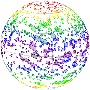
Example Poly4 plot
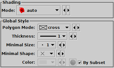
Poly4 form configuration panel
Configuration options are:
outline:
draws a line round the outside of the polygonfill:
fills the interior of the polygoncross:
draws a line round the outside of the polygon
and lines between all the verticesThe Mark4 form ( )
is available from the
Quad Position layer control,
and plots 4 similar markers of fixed size and shape representing
4 separate positions from the same table row.
This is a convenience (you could do the same thing by plotting
the four markers separately) that makes it easy to mark the corners of
polygons plotted from the Quad layer control.
)
is available from the
Quad Position layer control,
and plots 4 similar markers of fixed size and shape representing
4 separate positions from the same table row.
This is a convenience (you could do the same thing by plotting
the four markers separately) that makes it easy to mark the corners of
polygons plotted from the Quad layer control.
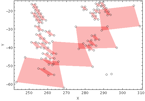
Example Mark4 plot
Mark4 form configuration panel
Configuration options are the same as for Mark:
The Area form ()
is available from the
Area layer control,
and outlines or fills areas that are defined in a table row.
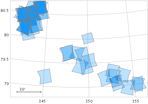
Example Area plot
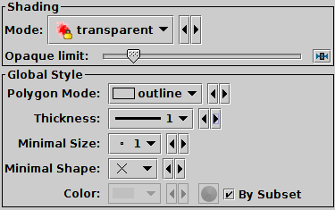
Area form configuration panel
Configuration options are:
outline:
draws a line round the outside of the polygonfill:
fills the interior of the polygoncross:
draws a line round the outside of the polygon
and lines between all the verticesThe Central form ()
is available from the
Area layer control,
and plots a point at the nominal center of the given area.
The effect is just the same as for the Mark form,
but it can be used from the Area layer control rather than
having to specify positional coordinates separately.
The plotted position is determined by the plotting code from the
shape information; it may or may not correspond to the shape's actual center.
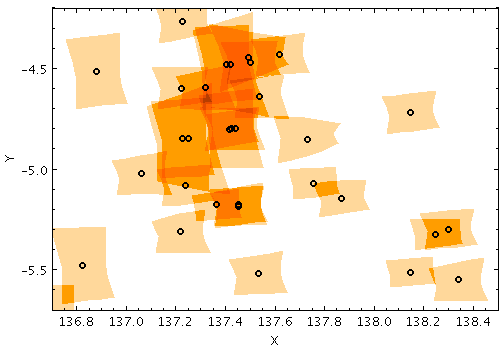
Example Central plot
Central form configuration panel
Configuration options are:
The AreaLabel form ()
is available from the
Area layer control,
and draws a text label near the nominal center of each plotted area.
The effect is just the same as for the Label form,
but it can be used from the Area layer control rather than
having to specify positional coordinates separately.
The plotted position is determined by the plotting code from the
shape information; it may or may not correspond to the shape's actual center.
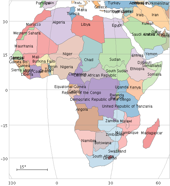
Example AreaLabel plot
AreaLabel form configuration panel
The configuration options are:
The Lines form (),
available from the
XYArray Layer Control,
draws a point-to-point line joining all the elements of X, Y
array-valued coordinates, resulting in one line for each table row.
It is typically used to plot a number of spectra or time series.
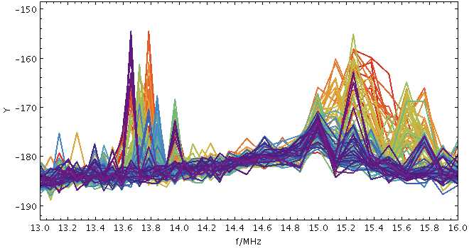
Example Lines plot
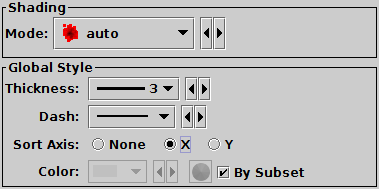
Lines form configuration panel
The configuration options are:
The Marks form (),
available from the
XYArray Layer Control,
draws a set of points representing all the elements of X, Y
array-valued coordinates, resulting in a sequence of points
for each table row.
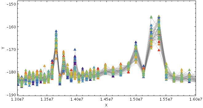
Example Marks plot
Mark form configuration panel
The configuration options are:
The Handles form (),
available from the
XYArray Layer Control,
draws a single pointer (a "handle") somewhere near each group of points
defined by pair of X/Y array coordinates.
This doesn't do much to show the shape of the line formed by the
array values, but it does provide a reference point for each line.
This can be used by the parts of TOPCAT that associated a fixed
position with each table row, in particular:
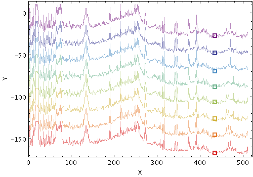
Example Handles plot
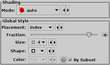
Handles form configuration panel
The configuration options are:
index:
(X,Y) position at a certain fraction of the way through the arrays,
as given by the Fraction value;
Fraction=0.0 is the first element, Fraction=1.0 is the lastymax:
(X,Y) position at which the maximum Y value is located
(Fraction is ignored)ymin:
(X,Y) position at which the minimum Y value is located
(Fraction is ignored)xmax:
(X,Y) position at which the maximum X value is located
(Fraction is ignored)xmin:
(X,Y) position at which the minimum X value is located
(Fraction is ignored)xymean:
center of gravity of all the (X,Y) points
(Fraction is ignored)The YErrors form (),
available from the
XYArray Layer Control,
draws a set of symmetric or asymmetric vertical error bars
representing all the elements of X, Y
array-valued coordinates, resulting in a sequence of error bars
for each table row.
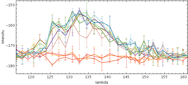
Example YErrors plot
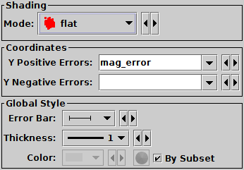
YErrors form configuration panel
The configuration options are:
The column names or expressions used here must be array values, matching the length of the data array values. If you need to create or manipulate array values, the functions in the Arrays class may be of use here.
The XYErrors form (),
available from the
XYArray Layer Control,
draws a set of error bars representing all the elements of X, Y
array-valued coordinates, resulting in a sequence of error bars
for each table row.
Symmetric or asymmetric vertical and/or horizontal error bars may be drawn,
and the shape of the error "bars" is quite configurable,
including error ellipses, rectangles etc.
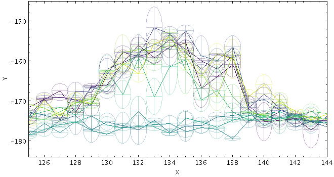
Example XYErrors plot
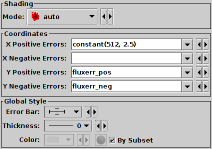
XYErrors form configuration panel
The configuration options are:
The column names or expressions used here must be array values, matching the length of the data array values. If you need to create or manipulate array values, the functions in the Arrays class may be of use here.
The StatLine form (),
available from the
XYArray Layer Control,
plots a single line based on a combination (typically the mean) of
input array-valued coordinates. The input X and Y coordinates must be
fixed-length arrays of length N; a line with N points is plotted, each
point representing the mean (or median, minimum, maximum, ...) of all
the input array elements at the corresponding position.
Note that because the X and Y arrays must be of a fixed size for all rows, and because combination is performed in both X and Y directions, this is typically only suitable for plotting combined spectra if they all share a common horizontal axis, e.g. are all sampled into the same wavelength bins. To visually combine spectra with non-uniform sampling, the ArrayQuantile form may be more useful.
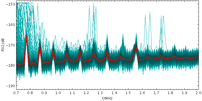
Example StatLine plot
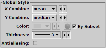
StatLine form configuration panel
The configuration options are:
mean:
the mean of the combined valuesmedian:
the median of the combined values (may be slow)min: the minimum of all the combined valuesmax: the maximum of all the combined valuesq.01:
the 1st percentile of the combined values (may be slow)q1:
the first quartile of the combined values (may be slow)q3:
the third quartile of the combined values (may be slow)q.99:
the 99th percentile of the combined values (may be slow)stdev:
the sample standard deviation of the combined valuessum: the sum of all the combined valuescount: the number of non-blank valuesThe StatMark form (),
available from the
XYArray Layer Control,
plots a set of markers based on a combination (typically the mean)
of input array-valued coordinates. The input X and Y coordinates must
be fixed-length arrays of length N; N markers are plotted, each one
representing the mean (or median, minimum, maximum, ...) of all the
input array elements at the corresponding position.
Note that because the X and Y arrays must be of a fixed size for all rows, and because combination is performed in both X and Y directions, this is typically only suitable for plotting combined spectra if they all share a common horizontal axis, e.g. are all sampled into the same wavelength bins. To visually combine spectra with non-uniform sampling, the ArrayQuantile form may be more useful.
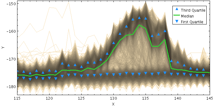
Example StatMark plot
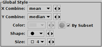
StatLine form configuration panel
The configuration options are:
mean:
the mean of the combined valuesmedian:
the median of the combined values (may be slow)min: the minimum of all the combined valuesmax: the maximum of all the combined valuesq.01:
the 1st percentile of the combined values (may be slow)q1:
the first quartile of the combined values (may be slow)q3:
the third quartile of the combined values (may be slow)q.99:
the 99th percentile of the combined values (may be slow)stdev:
the sample standard deviation of the combined valuessum: the sum of all the combined valuescount: the number of non-blank valuesThe ArrayQuantile form (),
available from the
XYArray Layer Control,
displays a quantile or quantile range for a set of plotted X/Y array pairs.
If a table contains one spectrum per row in array-valued wavelength
and flux columns, this plotter can be used to display a median of all
the spectra, or a range between two quantiles. Smoothing options are
available to even out noise arising from the pixel binning.
For each row, the X Values and Y Values arrays must be the same length as each other, but this plot type does not (unlike StatMark and StatLine) require the arrays to be sampled into the same bins for each row.
The algorithm calculates quantiles for all the X,Y points plotted in each column of pixels. This means that more densely sampled spectra have more influence on the output than sparser ones.
Note: In the current implementation, depending on the details of the configuration and the data, there may be some distortions or missing graphics near the edges of the plot. This may be improved in future releases, depending on feedback.
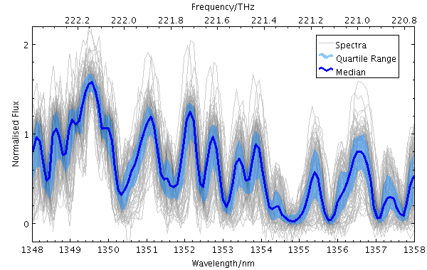
Example ArrayQuantile plot
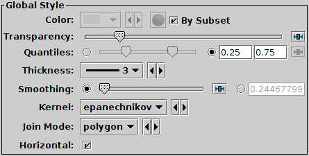
ArrayQuantile form configuration panel
The configuration options are:
The radio buttons let you toggle between using the slider to set the quantile value(s) or entering them in the text fields. If the two values are identical, you can leave the second text field blank.
You can adjust it using the slider (wider smoothing to the right) or enter a value in data coordinates explicitly in the text field. If the smoothed axis is logarithmic, the value is a multiplication factor rather than an additive increment.
The available options are:
The available options are:
Most of the Plot Forms have a style colour associated with them for each data set. This defines the basic colour used to plot the shape at each data point. However, many of the forms also ask you to select a Shading Mode, which determines the actual colour displayed in the plot for the plotted points. The shaded colour is based on the selected style colour, but may also be influenced by the number of points plotted there, some extra data coordinate, or other configuration information.
When exporting plots to an external vector graphics format (PDF, SVG or EPS), some of the shading modes may not behave the same as in a bitmap (on the screen, or to a bitmapped format such as GIF or PNG). Any such anomalies are noted in the in the mode descriptions below.
The different mode shading mode options are described in the following subsections.
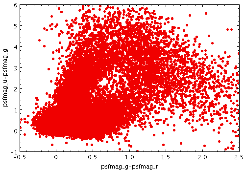
Example Flat shading mode plot
Flat shading mode selection
The Flat shading mode ( )
simply colours points in the colour selected by their style.
It has no additional parameters or coordinates.
)
simply colours points in the colour selected by their style.
It has no additional parameters or coordinates.
Exporting: This mode works without problem for both bitmapped and vector output.
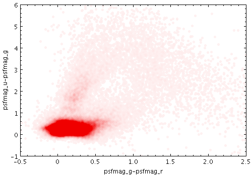
Example Translucent shading mode plot

Translucent shading mode selection
The Translucent shading mode ( )
colours shapes in a transparent version of the
colour selected by their style.
The degree of transparency is determined by how many points are
currently being plotted on top of each other,
and by the Transparency Level slider;
as you slide further to the right, points get more transparent.
Unlike transparent mode,
the transparency varies according to the current point density,
so you can usually leave the setting the same as you zoom
in and out.
)
colours shapes in a transparent version of the
colour selected by their style.
The degree of transparency is determined by how many points are
currently being plotted on top of each other,
and by the Transparency Level slider;
as you slide further to the right, points get more transparent.
Unlike transparent mode,
the transparency varies according to the current point density,
so you can usually leave the setting the same as you zoom
in and out.
Exporting: When the points are opaque, this mode works without problem for both bitmapped and vector output, but when the transparency is set there may be anomalies. Transparent points are rendered in PDF output, though the transparency levels may not be exactly the same as on the screen. This can be fixed by using the Force Bitmap option in the Plot Export dialogue. For PostScript, transparent points are rendered as opaque. You can use Force Bitmap with PostScript which will get transparency right for this layer, but then any earlier layers will be completely obscured.
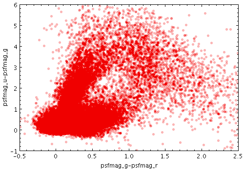
Example Transparent shading mode plot
Transparent shading mode selection
The Transparent shading mode ( )
colours shapes in a transparent version of the
colour selected by their style.
The degree of transparency is determined by the
Opaque Limit slider - at the left end,
points are fully opaque and this is equivalent to
Flat mode,
and as you slide further to the right,
the points get more transparent.
The higher the opaque limit, the more points have to be plotted
on top of each other to reach colour that fully obscures the background.
Unlike translucent mode,
transparency of each colour is fixed by the opaque limit,
rather than adjusting depending on the density of points currently plotted.
)
colours shapes in a transparent version of the
colour selected by their style.
The degree of transparency is determined by the
Opaque Limit slider - at the left end,
points are fully opaque and this is equivalent to
Flat mode,
and as you slide further to the right,
the points get more transparent.
The higher the opaque limit, the more points have to be plotted
on top of each other to reach colour that fully obscures the background.
Unlike translucent mode,
transparency of each colour is fixed by the opaque limit,
rather than adjusting depending on the density of points currently plotted.
Exporting: When the points are opaque, this mode works without problem for both bitmapped and vector output, but when the transparency is set there may be anomalies. Transparent points are rendered in PDF output, though the transparency levels may not be exactly the same as on the screen. This can be fixed by using the Force Bitmap option in the Plot Export dialogue. For PostScript, transparent points are rendered as opaque. You can use Force Bitmap with PostScript which will get transparency right for this layer, but then any earlier layers will be completely obscured.
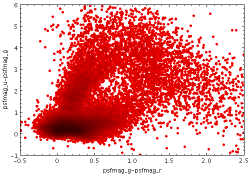
Example Auto shading mode plot
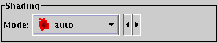
Auto shading mode selection
The Auto shading mode ( )
colours isolated points in their selected colour,
but where multiple points from the same data set
overlap it adjusts the colour by darkening it.
This means for that isolated points
(most or all points in a non-crowded plot, or outliers in a crowded plot)
it behaves just like Flat mode,
but it's easy to see where overdense regions lie.
)
colours isolated points in their selected colour,
but where multiple points from the same data set
overlap it adjusts the colour by darkening it.
This means for that isolated points
(most or all points in a non-crowded plot, or outliers in a crowded plot)
it behaves just like Flat mode,
but it's easy to see where overdense regions lie.
This is like Density mode, but with no user-configurable options.
This is the default mode for 2d plots, since it gives you a good first idea of what the data is doing. For 3d plots it can be used, and it works well for single dataset plots, but in the case of multiple datasets it can be misleading since the coloured pixels can't be placed sensibly in the 3d space.
The colour darkening is based on the asinh function; the intention is that two points overlaid should be just enough different in colour for the difference to be visible, and the mapping is scaled so that if there are very dense regions they will come out nearly black.
Exporting: When exported to vector formats, the output is automatically forced to a bitmap for Auto-mode layers. In the case of PostScript, this completely obscures any previous layers.
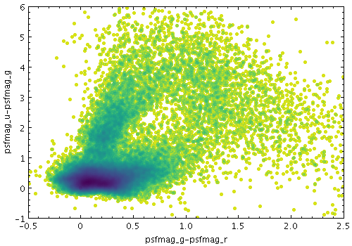
Example Density shading mode plot
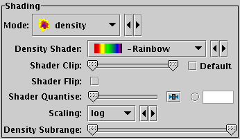
Density mode selection
The Density shading mode ( )
uses a configurable colour map
to indicate how many points are plotted over each other.
Specifically, it colours each pixel according to how many times that
pixel has has been covered by one of the shapes plotted by the layer
in question.
To put it another way, it generates a false-colour density map
with pixel granularity using a smoothing kernel of the form of
the shapes plotted by the layer.
The upshot is that you can see the plot density of points or other
shapes plotted.
)
uses a configurable colour map
to indicate how many points are plotted over each other.
Specifically, it colours each pixel according to how many times that
pixel has has been covered by one of the shapes plotted by the layer
in question.
To put it another way, it generates a false-colour density map
with pixel granularity using a smoothing kernel of the form of
the shapes plotted by the layer.
The upshot is that you can see the plot density of points or other
shapes plotted.
This is like Auto mode, but with more user-configurable options. The options are:
Although these options give you quite some control over how densities are mapped to colours, this mode does not display the colour mapping in a way that shows you quantitatively which colours correspond to which numeric density values. If you want that kind of visual feedback, you should use the Weighted shading mode, which can be configured to display point densities (as well as other quantities), and also causes a colour ramp to be displayed under control of the Aux Axis control.
Exporting: When exported to vector formats, the output is automatically forced to a bitmap for Density-mode layers. In the case of PostScript, this completely obscures any previous layers.
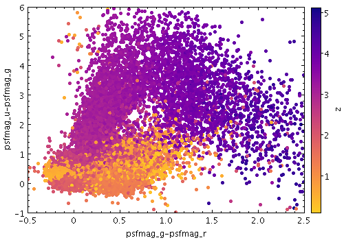
Example Aux shading mode plot
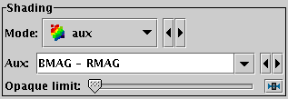
Aux mode selection
The Aux shading mode ( )
colours each point according to the value of an additional
data coordinate, using a colour map shared with other layers in the plot.
The point colours then represent an additional dimension.
There is an additional option to draw the points with a fixed transparency.
)
colours each point according to the value of an additional
data coordinate, using a colour map shared with other layers in the plot.
The point colours then represent an additional dimension.
There is an additional option to draw the points with a fixed transparency.
The shading is done using the shared colour map. This colour map is used by all currently visible Aux, Weighted, Grid and SkyDensity layers. When at least one such layer is being plotted, the Aux Axis control is visible in the control panel, which allows you to configure the colour map, range, ramp display etc.
The options are:
Exporting: Transparent points are rendered in PDF output, though the transparency levels may not be exactly the same as on the screen. This can be fixed by using the Force Bitmap option in the Plot Export dialogue. For PostScript, transparent points are rendered as opaque. You can use Force Bitmap with PostScript which will get transparency right for this layer, but then any earlier layers will be completely obscured.
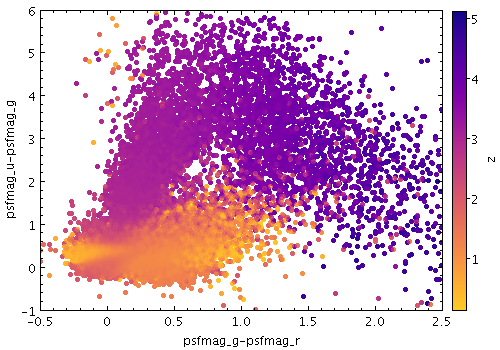
Example Weighted shading mode plot
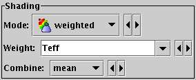
Weighted mode selection
The Weighted shading mode ( )
paints markers using colours indicating density at each pixel like
the Density mode, but with an optional weighting coordinate,
using a colour map shared with other layers in the plot.
You can configure how the weighted coordinates are combined
at each pixel to give the final weighted result.
Depending on the configuration and actual point density,
this can behave
in some ways like Aux mode and
in some ways like Density mode,
but allows you to do things that are not possible in either.
)
paints markers using colours indicating density at each pixel like
the Density mode, but with an optional weighting coordinate,
using a colour map shared with other layers in the plot.
You can configure how the weighted coordinates are combined
at each pixel to give the final weighted result.
Depending on the configuration and actual point density,
this can behave
in some ways like Aux mode and
in some ways like Density mode,
but allows you to do things that are not possible in either.
The shading is done using the shared colour map. This colour map is used by all currently visible Weighted, Aux, Grid and SkyDensity layers. When at least one such layer is being plotted, the Aux Axis control is visible in the control panel, which allows you to configure the colour map, range, ramp display etc.
The options are:
The following options (some are more useful than others) are currently available:
sum: the sum of all weightsmean: the mean of all weightsmedian: the median of all weights (may be slow)q1: the first quartile of all weights (may be slow)q3: the third quartile of all weights (may be slow)min: the minimum weightmax: the maximum weightstdev: the sample standard deviation of all weightscount: the number of points plotted
(weight value is ignored, this is like Density mode)hit: one if any point is plotted, blank otherwise
(weight value is ignored, this is like Flat mode)Exporting: When exported to vector formats, the output is automatically forced to a bitmap for Density-mode layers. In the case of PostScript, this completely obscures any previous layers.
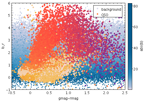
Example PAux shading mode plot
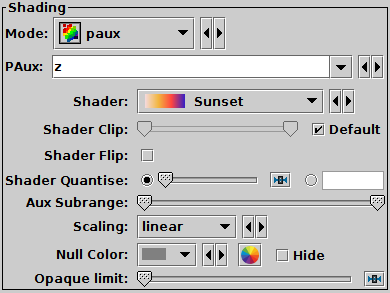
PAux mode selection
The PAux (private-auxiliary) shading mode ( )
colours each point according to the value of an additional data coordinate,
but using a private colour map.
The point colours then represent an additional dimension.
There is an additional option to draw the points with a fixed transparency.
)
colours each point according to the value of an additional data coordinate,
but using a private colour map.
The point colours then represent an additional dimension.
There is an additional option to draw the points with a fixed transparency.
This mode is like Aux mode, except that the colour map is not shared with other layers, and the colour ramp is not displayed. So, by using this mode alongside Aux or Weighted modes you can make a plot that uses multiple different colour maps, though only one can have an associated visible ramp.
The options are:
Exporting: Transparent points are rendered in PDF output, though the transparency levels may not be exactly the same as on the screen. This can be fixed by using the Force Bitmap option in the Plot Export dialogue. For PostScript, transparent points are rendered as opaque. You can use Force Bitmap with PostScript which will get transparency right for this layer, but then any earlier layers will be completely obscured.
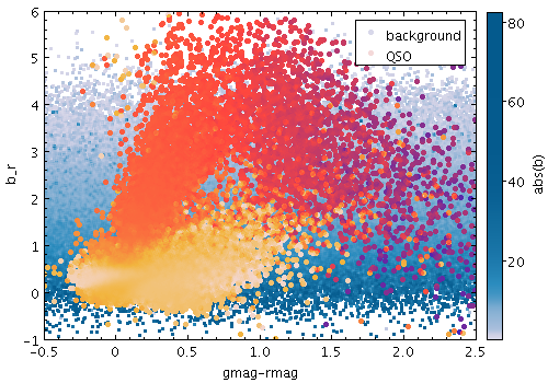
Example PWeighted shading mode plot
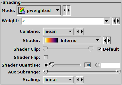
PWeighted mode selection
The PWeighted (private-weighted) shading mode
( )
paints markers using colour indicating weighted density at each pixel,
using a private colour map.
)
paints markers using colour indicating weighted density at each pixel,
using a private colour map.
This mode is like Weighted mode, except that the colour map is not shared with other layers, and the colour ramp is not displayed. So, by using this mode alongside Aux or Weighted modes you can make a plot that uses multiple different colour maps, though only one can have an associated visible ramp.
The options are:
The following options (some are more useful than others) are currently available:
sum: the sum of all weightsmean: the mean of all weightsmedian: the median of all weights (may be slow)q1: the first quartile of all weights (may be slow)q3: the third quartile of all weights (may be slow)min: the minimum weightmax: the maximum weightstdev: the sample standard deviation of all weightscount: the number of points plotted
(weight value is ignored, this is like Density mode)hit: one if any point is plotted, blank otherwise
(weight value is ignored, this is like Flat mode)Exporting: When exported to vector formats, the output is automatically forced to a bitmap for PWeighted-mode layers. In the case of PostScript, this completely obscures any previous layers.
A number of colour maps are available, and used for instance with the Aux Axis Control and Density Shading Mode. Not all colour maps are suitable/available in all contexts, and in some cases the maps are by default clipped at one end to avoid for instance white-on-white plotting, but the lists below give an overview of which named colourmaps can be used.
The absolute colour maps are listed below: these do not depend on the underlying colour of the plotted symbols, so are suitable when only one dataset is being plotted.

Absolute colour maps
The non-absolute colour maps are listed below: these modify an underlying colour, so are suitable for applying to several different datasets with different underlying colours. The representation here shows how they affect several different colours; for each row of pixels the unmodified (value=0) colour is at the left of the image and the most modified (value=1) is at the right.

Non-absolute colour maps
These colour maps have been derived from several sources, including SkyCat/GAIA, MatPlotLib 1.5, Gnuplot, Daniel Michalik, Paul Tol, CMasher, Color Brewer, HCL Wizard, Dave Green, xkcd, and maybe some others I forgot.
It is also possible to set up custom colour maps by using the
lut.files
System Property.
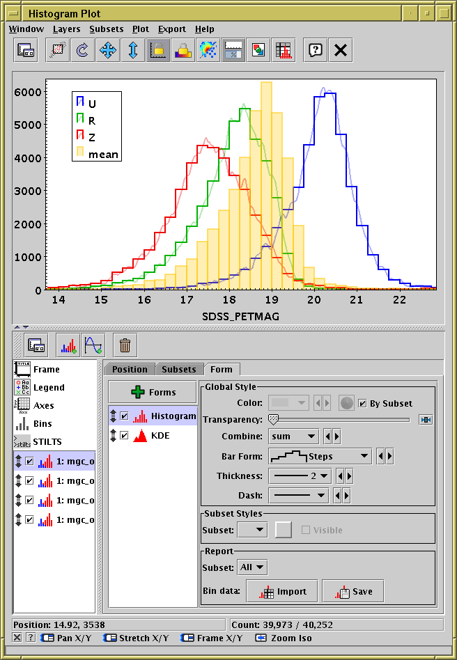
Histogram Plot Window
The Histogram Plot ()
plots 1-dimensional histograms and some variants on the idea of a
1-dimensional Kernel Density Estimate.
In many respects it works like the Plane Plot,
but it has a restricted set of plot types
and an additional fixed control
Bins,
and the scrolling works a bit differently.
See the Window Overview for features common to all plotting windows.
As well as the standard actions, this window additionally provides the following toolbar buttons:
Measure Distance
In addition, the histogram window lets you export the binned data as a new table, either saving it or loading it directly into TOPCAT's table list. The following actions are available in the Export menu; note they only apply to histograms proper, not to KDEs:
 Save as Table
 Import as Table
The Histogram Plot offers the following plot controls:
Histogram Layer Control, with these form options:
Function Layer Control
The following subsections describe navigation, axis configuration and bin configuration.
For general comments on plot navigation, see Appendix A.4.2.1. Additional configuration options are available in the Navigation tab of the Axes control.
The navigation actions for this window are:
Left drag
Right drag (CTRL-drag)
Zooming horizontally will normally adjust the width of the histogram bars appropriately.
Normally, the zoom will be centered horizontally at the mouse position and vertically on the X axis, so the zoom will not move the bottom of the histogram. You can adjust that with the Anchor X/Y Axis options in the Navigation axis configuration tab.
Wheel
You can also manually fix the plot bounds using the Range tab of the Axes control.
The Histogram Plot axis control is very similar to the Plane Plot axis control described in Appendix A.4.9.2. The only difference is in the Navigation tab. For the histogram, the Anchor X Axis option is set on by default, since you will usually want the Y=0 line to stay anchored to the bottom of the plot when zooming.
The Bins control ()
is found in the control stack of the
Histogram window.
It configures the common placement and calculation of some options
for all the histogram-like layers displayed.
Being able to set these values in common for all displayed layers
of a similar type can be convenient, but if you need to use different
parameters for different datasets, you can plot the same layer forms
in the Plane window
(which has no fixed Bins control) instead.
There are three tabs: Histogram, KDE and General, described below.
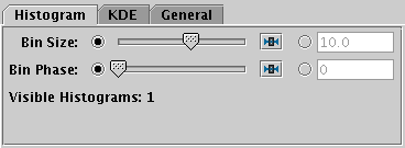
Histogram tab of histogram window Bins fixed control
The Histogram tab affects all Histogram layers, and to some extent the Gaussian layer, and has the following controls:
Although Gaussian layers don't have bars, the value of this control can affect the scaling of plotted gaussian fits for some normalisation options, since the Gaussian plots try to scale themselves to match the height of corresponding histograms.
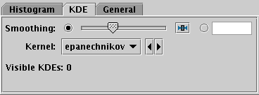
KDE tab of histogram window Bins fixed control
The KDE (Kernel Density Estimate) tab affects all KDE, KNN and Densogram layers, and has the following controls:
Sliding the slider to the right makes the kernel width larger. The width in data units is shown in the text field on the right (if the X axis is logarithmic, this is a factor). Alternatively you can click the radio button near the text field, and enter the width in data units directly.
Note this affects KDE and Densogram layers, but not KNN layers, which have their own smoothing controls.
The available options are:
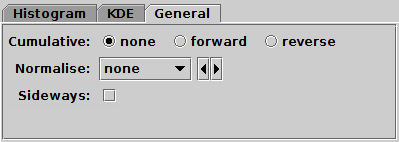
General tab of histogram window Bins fixed control
The General tab affects all histogram-like layers, and has the following controls:
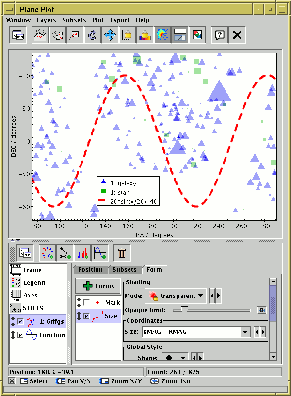
Plane Plot Window
The Plane Plot ()
plots 2-dimensional Cartesian positions on a plane.
The positional coordinates are X and Y.
To control the direction and linear/log scaling of the axes,
see the Coords tab of the
Axes control.
The Plane Plot offers the following plot controls:
Position Layer Control, with these form options:
Pair Layer Control, with these form options:
Area Layer Control, with these form options:
Quad Layer Control, with these form options:
XYArray Layer Control, with these form options:
Histogram Layer Control, with these form options:
Function Layer Control
As well as the standard actions, this window additionally provides the following toolbar buttons:
and Subsets menu itemSee the Window Overview for features common to all plotting windows. The following subsections describe navigation and axis configuration.
For general comments on plot navigation, see Appendix A.4.2.1. Additional configuration options are available in the Navigation tab of the Axes control.
The navigation actions for this window are:
Left drag
Right drag (CTRL-drag)
Center drag (SHIFT-drag)
Wheel
Left click
You can also manually fix the plot bounds using the Range tab of the Axes control.
The Axes control () for the
plane plot window has the following tabs:
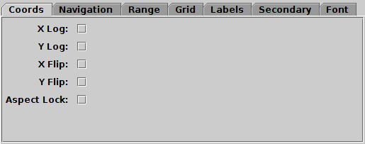
Coords tab of plane Axes control
The Coords tab controls the axis coordinates. It has the following options:
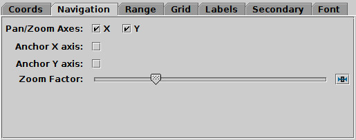
Navigation tab of plane Axes control
The Navigation tab controls details of how the navigation works. It has the following options:
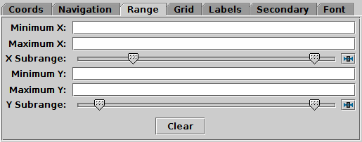
Range tab of plane Axes control
The Range tab provides manual configuration of the visible range of the plot. Making changes to this tab will reset the visible plot range, but not vice versa - zooming and panning in the usual way will not change the settings of this panel.
Filling in the Minimum/Maximum fields for either or both axes will constrain the corresponding range of the visible data. The limits corresponding to any of those fields that are left blank will initially be worked out from the data. The Subrange double-sliders restrict the ranges within the (explicit or automatic) min/max ranges. Note you can move both sliders at once by grabbing a position between the two.
The Clear button resets all the fields.
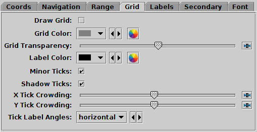
Grid tab of plane Axes control
The Grid tab configures the appearance of the axis grid. It has the following options:
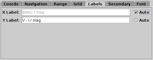
Labels tab of plane Axes control
The Labels tab controls the text labels on the axes. If the Auto checkbox is set, the text will be taken from one of the data coordinates being plotted on that axis. To override those with your own axis labels, unset Auto and type text in to the Label fields.
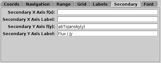
Secondary tab of plane Axes control
The Secondary tab controls optional secondary X and Y axes at the top and right edges of the plot, to go with the standard (primary) X and Y axes at the bottom and left edges, so you can annotate a plot for instance with both magnitudes and fluxes, or both frequency and wavelength.
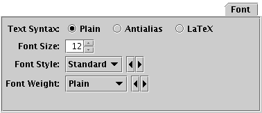
Font tab
The Font tab configures the font used for axis annotation. It also affects some other things like the legend.
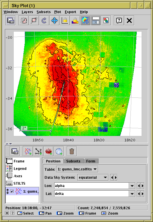
Sky Plot Window
The Sky Plot ()
plots longitude/latitude positions onto the celestial sphere.
It can plot to a number of projections
(currently Sin, Hammer-Aitoff and Plate Carrée).
The positional coordinates are Longitude and Latitude, specified in degrees. When supplying them, you can specify an associated Data Sky System (Equatorial, Galactic, Supergalactic or Ecliptic2000). Note that this is the sky system of the data coordinates, not (necessarily) of the plot you want to see. To specify the coordinates you want the data to be plotted on, use the View Sky System option in the Projection tab of the Axes control. However, if you just want to view the data using the same system as the coordinates you are supplying, you can ignore leave these values as their default (both Equatorial) and no conversion will be done.
The sky plot offers the following plot controls:
Position Layer Control, with these form options:
Pair Layer Control, with the following plot controls:
Area Layer Control, with the following plot controls:
Quad Layer Control, with the following plot controls:
Healpix Layer Control
SkyGrid Layer Control
As well as the standard actions, this window additionally provides the following toolbar buttons:
See the Window Overview for features common to all plotting windows. The following subsections describe navigation and axis configuration.
For general comments on plot navigation, see Appendix A.4.2.1. Additional configuration options are available in the Navigation tab of the Axes control.
The navigation options for this window are:
Left drag
The Hammer-Aitoff and Plate Carrée projections act like a piece of paper that can be dragged around in two dimensions in the usual way.
Wheel
Right drag (CTRL-drag)
Center drag (SHIFT-drag)
Left click
You can also navigate to a known sky position by coordinates or object name using the FOV tab of the Axes control.
The Axes control () for the
sky plot window has the following tabs:
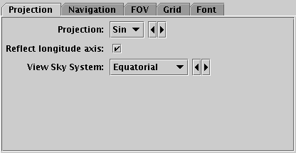
Projection tab of the sky Axes control
The Projection tab controls how the sky position coordinates are projected onto the screen.
       x = [2sqrt(2)/sqrt(1+cos(lat)cos(lon/2))]cos(lat)sin(lon/2)
       y = [sqrt(2)/sqrt(1+cos(lat)cos(lon/2))]sin(lat)
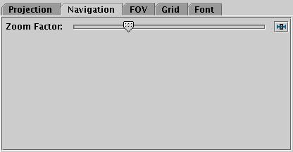
Navigation tab of sky Axes control
The Navigation tab controls details of how the navigation works. It has the following option:
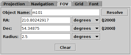
Field Of View tab of the sky Axes control
The FOV (Field Of View) tab allows you to enter a sky position or object name and a radius and positions the view at that region. Filling in the position and radius fields and hitting return will reposition the sky view, but not vice versa; normal pan/zoom operations will not affect the content of this panel.
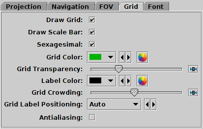
Grid tab of the sky Axes control
The Grid tab controls how the sky coordinate axes appear.
Font tab
The Font tab configures the font used for axis annotation. It also affects some other things like the legend.
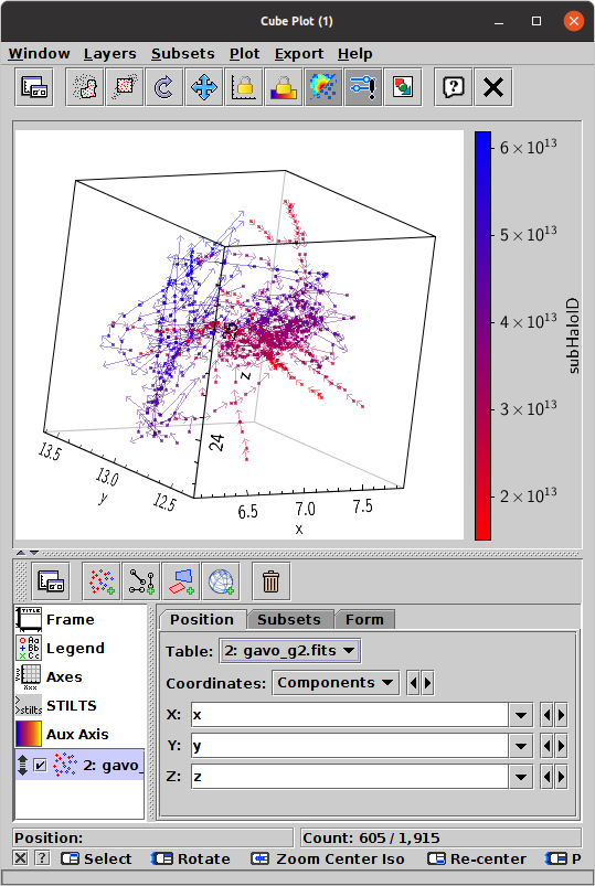
Cube Plot Window
The Cube Plot ()
plots 3-dimensional Cartesian positions in a 3-d space.
By default the positional coordinates are X, Y and Z, but the Coordinates selector lets you specify them in different ways:
To control the direction and linear/logarithmic scaling of the axes, see the Coords tab of the Axes control.
The cube plot offers the following plot controls:
Position Layer Control, with these form options:
Pair Layer Control, with the following plot controls:
Quad Layer Control, with the following plot controls:
SphereGrid Layer Control
As well as the standard actions, this window additionally provides the following toolbar button:
and Subsets menu item:Note that use of the Auto, Density and Weighted shading modes can be confusing in 3 dimensions with multiple datasets. This is because pixels based on density along a line of sight are not located at any point on that line, so shaded pixels can't appear at the "right" place in the 3-d space. The same applies to a lesser extent with contours. They work fine with a single dataset though.
See the Window Overview for features common to all plotting windows. The following subsections describe navigation and axis configuration.
For general comments on plot navigation, see Appendix A.4.2.1. Additional configuration options are available in the Navigation tab of the Axes control.
Navigation in three dimensions with a two-dimensional screen and mouse is a bit of a challenge. However, the actions listed below should make it fairly straightforward to navigate around points in 3d space to zoom in on the regions that you are interested in.
Left drag
Wheel
Right drag (CTRL-drag)
Center drag (SHIFT-drag)
Left click
In 3d, it's not obvious which is the nearest point to a 2d cursor, since a screen position represents a line not a point. To break the degeneracy, the point used is the one nearest the center of mass of plotted points along the line of sight represented by the cursor position. The upshot of this is that if you click on an isolated point, you'll pick that point, and if you click on a dense cluster, you'll get a point near the center (of mass) of that cluster.
Right click (CTRL-click)
You can also manually fix the plot bounds using the Range tab of the Axes control.
The Axes control () for the
cube plot window has the following tabs:
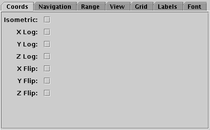
Coords tab of the cube Axes control
The Coords tab controls the axis coordinates. It has the following options:
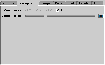
Navigation tab of the cube Axes control
The Navigation tab controls details of how the navigation works. It has the following options:
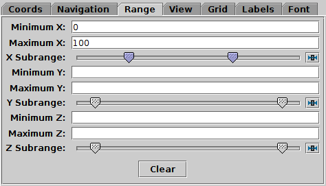
Range tab of the cube Axes control
The Range tab provides manual configuration of the visible range of the plot. Making changes to this tab will reset the visible plot range, but not vice versa - zooming and panning in the usual way will not change the settings of this panel.
Filling in the Minimum/Maximum fields for one or more axes will constrain the corresponding range of the visible data. The limits corresponding to any of those fields that are left blank will initially be worked out from the data. The Subrange double-sliders restrict the ranges within the (explicit or automatic) min/max ranges. Note you can move both sliders at once by grabbing a position between the two.
The Clear button resets all the fields.
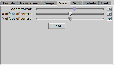
View tab of the cube Axes control
The View tab can configure how the cube containing the data is viewed in the plot window, though it does not control the content of the cube.
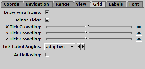
Grid tab of the cube Axes control
The Grid tab configures the appearance of the cube wire frame enclosing the data volume.
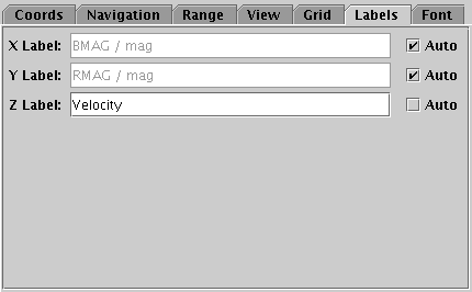
Labels tab of the cube Axes control
The Labels tab controls the text labels on the axes. If the Auto checkbox is set, the text will be taken from one of the data coordinates being plotted on that axis. To override those with your own axis labels, unset Auto and type text in to the Label fields.
Font tab
The Font tab configures the font used for axis annotation. It also affects some other things like the legend.
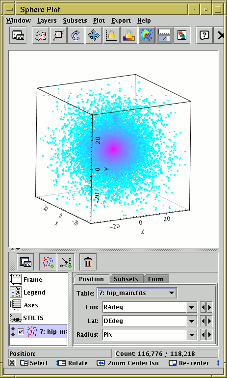
Sphere Plot Window
The Sphere Plot ()
plots spherical polar coordinates in an isotropic 3-dimensional space.
Although the supplied coordinates are spherical polar,
the visible space is not necessarily centred on the coordinate origin,
and the visible axes are Cartesian.
In many respects this works like the
Cube Plot Window
The positional coordinates are Longitude and Latitude (in degrees) and Radius.
The sphere plot offers the following plot controls:
Position Layer Control, with these form options:
Pair Layer Control, with the following plot controls:
Area Layer Control, with the following plot control:
Quad Layer Control, with the following plot controls:
SphereGrid Layer Control
See the Window Overview for features common to all plotting windows. The following subsections describe navigation and axis configuration.
For general comments on plot navigation, see Appendix A.4.2.1. Additional configuration options are available in the Navigation tab of the Axes control.
Navigation in three dimensions with a two-dimensional screen and mouse is a bit of a challenge. However, the actions listed below should make it fairly straightforward to navigate around points in 3d space to zoom in on the regions that you are interested in. The actions are quite like for the Cube Window, but all zooming is isotropic.
Left drag
Wheel
Right drag (CTRL-drag)
Center drag (SHIFT-drag)
Left click
In 3d, it's not obvious which is the nearest point to a 2d cursor, since a screen position represents a line not a point. To break the degeneracy, the point used is the one nearest the center of mass of plotted points along the line of sight represented by the cursor position. The upshot of this is that if you click on an isolated point, you'll pick that point, and if you click on a dense cluster, you'll get a point near the center (of mass) of that cluster.
Right click (CTRL-click)
You can also manually fix the plot bounds using the Range tab of the Axes control.
The Axes control () for the
sphere plot window has the following tabs:
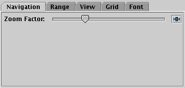
Navigation tab of the sphere Axes control
The Navigation tab controls details of how the navigation works. It has the following option:

Range tab of the sphere Axes control
The Range tab provides manual configuration of the data range of the plot. Making changes to this tab will reset the visible plot range, but not vice versa - zooming and panning in the usual way will not change the settings of this panel. Any values not filled in will be determined from the data. The fields are:
The Clear button resets all the fields.
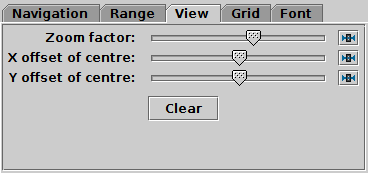
View tab of the sphere Axes control
The View tab can configure how the cube containing the data is viewed in the plot window, though it does not control the content of the cube.
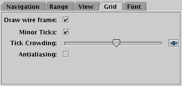
Grid tab of the sphere Axes control
The Grid tab configures the appearance of the cube wire frame enclosing the data volume.
Font tab
The Font tab configures the font used for axis annotation. It also affects some other things like the legend.
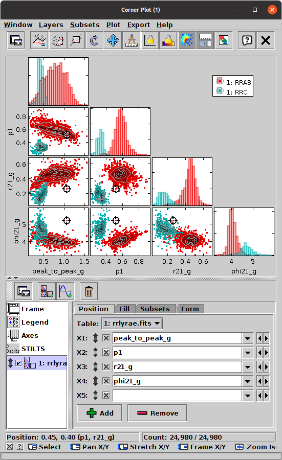
Corner Plot Window
The Corner Plot ()
represents the relationships between multiple quantities
by drawing a scatter-like plot of every pair of coordinates,
and/or a histogram-like plot of every single coordinate,
and placing these on (half or all of) a square grid.
The horizontal coordinates of all the plots on each column,
and the vertical coordinates of all the plots on each row,
are aligned.
The plots are all linked, so you can
make graphical selections
or click on a point to activate it
in one of the panels, and the other panels will immediately
reflect that action.
Single-coordinate (histogram-like) plots appear on the diagonal,
and coordinate-pair (scatter plot-like) plots appear off diagonal.
By default only the diagonal and sub-diagonal part of the resulting
plot matrix is shown, since the plots above the diagonal are equivalent
to those below it, but this is configurable.
This representation is variously known as a corner plot,
scatter plot matrix, splom or
pairs plot.
In principle any number of quantities can be simultaneously compared
in this way, but attempting to use too many will make
the individual plots too small to be useful.
Depending on the size of your screen, you may find about 20 is a
reasonable upper limit, though more detail will be visible with fewer.
Note that the Float Controls () button
(or equivalent action in the Window menu)
can be used to detach the control panel from the plot display and so
free up more space for the visualisation itself.
By default the linear size of the plot grid will be defined
by the highest-numbered non-blank coordinate that is visible
in any of the active Position layer controls,
but it can be adjusted directly in the Axes control
().
The configuration of the plots is done in the same way as for the Plane Plot, and many of the plot types that are available there can be used in the grid cells of this plot. The Corner Plot currently offers the following plot controls:
Matrix Layer Control, containing these scatter-plot like actions:
and these histogram-like actions:
The scatter-plot-like options will generate plots
in the off-diagonal positions of the grid,
and the histogram-like ones will generate plots on the leading diagonal.
By default the Mark and Histogram
options are both selected,
but you can hide these as well as adding others.
Function Layer Control; at present this draws the same function
in all visible grid positions, both off- and on-diagonal.
As well as the standard actions, this window additionally provides the following toolbar buttons:
See the Window Overview for features common to all plotting windows. The following subsections describe navigation and axis configuration.
Note: the Corner Plot Window is new at TOPCAT version 4.9. Some of the features are experimental and may be changed in future releases.
Navigation actions in the corner plot are the same as for the Plane Plot; you can pan and zoom on each panel in the grid of plots using the mouse. However in this case the action will affect not only the panel that you are pointing at, but all the other panels in the same row and the other panels in the same column, so that the horizontal and vertical axes stay consistent per row and per column.
Using the mouse to drag and zoom on one axis only, rather than both at once, by positioning it just outside the bounds of one of the panels (e.g. between panels) as described below, can be particularly useful in this plot.
The navigation actions are:
Left drag
Right drag (CTRL-drag)
Center drag (SHIFT-drag)
Wheel
Left click
The Axes control () for the
corner plot window has the following tabs:
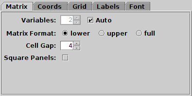
Matrix tab of corner Axes control
The Matrix tab configures the grid on which the individual plots are placed. It has the following options:
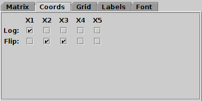
Coords tab of corner Axes control
The Coords tab controls the axis coordinates. For each currently visible axis there are two checkboxes:
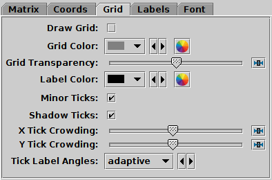
Grid tab of corner Axes control
The Grid tab configures the appearance of the axis grid in each panel. It has the following options:
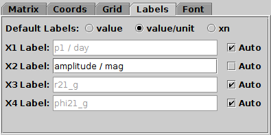
Labels tab of corner Axes control
The Labels tab controls the text labels on the axes. The axes are labelled according to the text listed for each coordinate X1, X2, .... By default these labels are assigned automatically, but you can override this by unchecking the Auto checkbox for the coordinate in question to enter your own text.
The automatically assigned values are generally taken by looking at the values entered into the coordinate selector fields of the Position tabs controlling the plot, but the details are determined by the Default Labels selector. This has three options:
Font tab
The Font tab configures the font used for axis annotation. It also affects some other things like the legend.
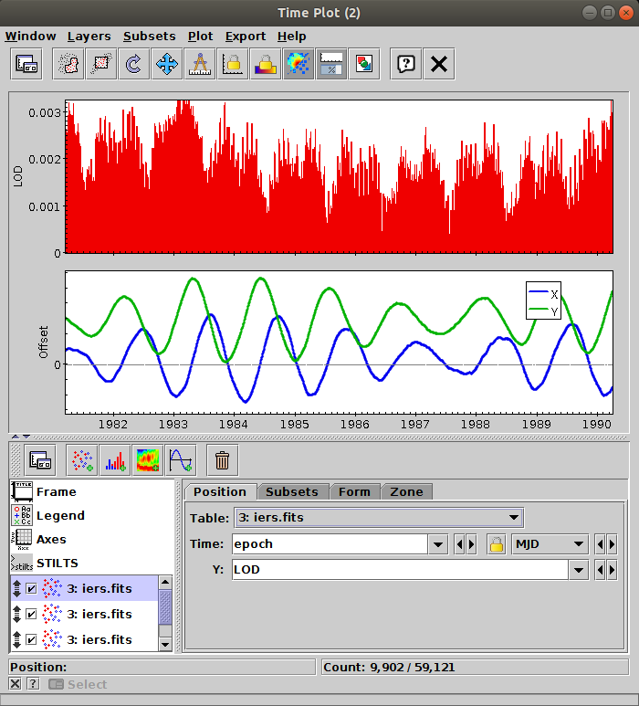
Time Plot Window
The Time Plot ()
is intended for plotting time series data.
The horizontal axis represents time, and can be labelled accordingly (for instance in minutes, hours, days, months and years), and the window can display appropriate types of plot including spectrograms.
To define the time coordinate, use the Time selector in position tabs as usual. Note however that this contains a time format selector on the right hand side that indicates how the selected quantity will be interpreted as a time value. The options are:
).
Unlike most of the other plot windows the Time plot can display different data plots in different plot Zones stacked vertically on top of each other, so that different plots share a time axis but have their own Y axis. The vertical spacing between the stacked plots can be configured using the Cell Gap configuration option in in the Spacing tab of the Frame Control.
It is possible to abuse this plot type to stack plots that do not actually have time on the horizontal axis. To do that, select mjd as the Time Format in the Grid tab of the Axes Control, and make sure that any time format selectors (described above) are similarly set to MJD. You may need to check that the right Zone is chosen (usually the bottom one) when you configure the axes.
The Time Plot offers the following plot controls:
Position Layer Control, with these form options:
Line
Linear Fit
Mark
Error Bars (vertical bars only) Label
Fill
Quantile
Grid
Histogram Layer Control with these form options:
Note that some of these histogram-like controls offer the
Combine option that lets you define how values
are combined together.
If you choose the sum-per-unit
or count-per-unit
options, you can also use the Per Unit selector
to determine whether values are represented as sums/counts per
second, hour, day, year, etc.
Spectrogram Layer Control
Function Layer Control
As well as the standard actions, this window additionally provides the following toolbar button:
See the Window Overview for features common to all plotting windows. The following subsections describe zones, navigation and axis configuration.
Unlike the other plot types, the Time plot can display data in multiple panels, known as Zones, stacked vertically. All plots therefore share the same time axis, but can have different Y axes.
By default, each new plot added is displayed in a new zone stacked beneath the existing ones. By using the Zone tab for each plot however, you can control which plots appear in which zones. Each zone has a numeric identifier, which by default increments by one for each new plot, but if you select the same identifier for several plots, they will all appear in the same zone.
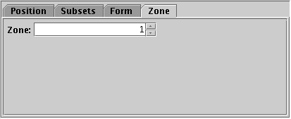
Zone selection tab
Some of the fixed controls
(Axes and
Aux )
operate on a per-zone basis.
If multiple zones are visible, then a zone selector is displayed
above the tabs:
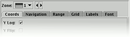
Zone selector for Axes Control
In this case you should select the zone you want to control and adjust the configuration for that zone only. The selector shows an icon indicating the position of the zone in question. Each zone has to be configured separately. In a future release a global zone configuration option may be introduced as well.
This multi-zone feature is currently available only for the Time plot, but it may be added to other plot types at some point in the future.
For general comments on plot navigation, see Appendix A.4.2.1. Additional configuration options are available in the Navigation tab of the Axes control.
Horizontal navigation (panning and zooming left and right along the shared time axis) affects all the stacked zones, but vertical navigation (panning and zooming along the Y axis of each zone) is done independently for each zone.
The navigation actions for this window are:
Left drag
Right drag (CTRL-drag)
Center drag (SHIFT-drag)
Wheel
Left click
You can also manually fix the plot bounds using the Range tab of the Axes control.
Note: the Time Plot has multiple plot Zones, and the axes are configured individually for each zone.
The Axes () control for the
time plot window has the following tabs:
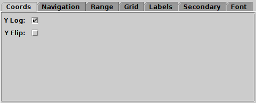
Coords tab of time Axes control
The Coords tab controls the vertical axis coordinates (you can't flip or rescale the time axis). It has the following options:
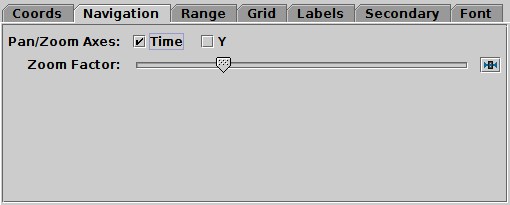
Navigation tab of time Axes control
The Navigation tab controls details of how the navigation works. It has the following options:
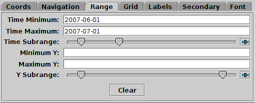
Range tab of time Axes control
The Range tab provides manual configuration of the visible range of the plot. Making changes to this tab will reset the visible plot range, but not vice versa - zooming and panning in the usual way will not change the settings of this panel.
Filling in the Minimum/Maximum fields for either or both axes will constrain the corresponding range of the visible data. The limits corresponding to any of those fields that are left blank will initially be worked out from the data. The Subrange double-sliders restrict the ranges within the (explicit or automatic) min/max ranges. Note you can move both sliders at once by grabbing a position between the two. For the time axis, the range may be entered as an ISO-8601 date/time value.
The Clear button resets all the fields.
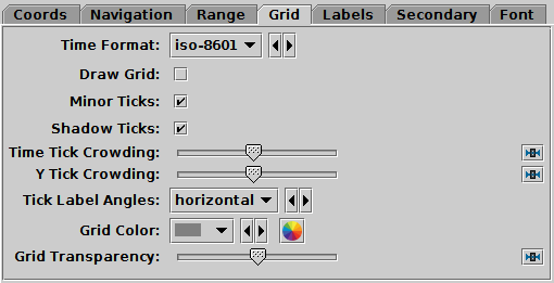
Grid tab of time Axes control
The Grid tab configures the appearance of the axis grid. It has the following options:
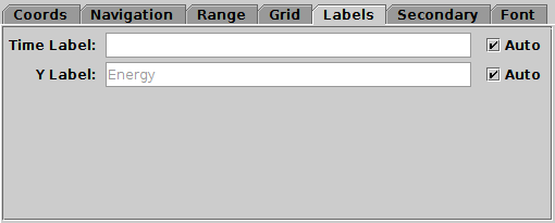
Labels tab of time Axes control
The Labels tab controls the text labels on the horizontal and vertical axes. If the Auto checkboxes are set, the Time axis will be unlabelled, and the Y axis label will be taken from one of the data coordinates being plotted on the Y axis. To override those with your own axis labels, unset Auto and type text in to the field.
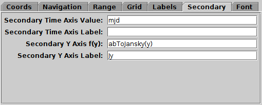
Secondary tab of time Axes control
The Secondary tab controls optional secondary Time and Y axes at the top and right edges of the plot, to go with the standard (primary) Time and Y axes at the bottom and left edges, so for instance you can annotate the vertical dimension with both magnitudes and flux, or the horizontal dimension with both decimal year and MJD.
mjd: Modified Julian Datejd: Julian DaydecYear: decimal year CEunixSec: seconds since 1970-01-01T00:00:00
Font tab
The Font tab configures the font used for axis annotation. It also affects some other things like the legend.
This section describes the old-style plotting windows used as standard in TOPCAT versions 2 and 3. Since version 4 (2013), the visualisation has been rewritten, and the new standard plotting windows are described in Appendix A.4. The windows described in this section are mildly deprecated, and will not be developed further. Most of their capabilities are handled better by the new-style plotting windows. However, these ones are still functional and if you want to use them you can find them in the Graphics menu of the Control Window, below the new-style plot options.
Common features of the old-style plotting windows are described in the first subsection below; the specific windows themselves are described in the later subsections.
The various types of old-style plotting windows have different characteristics to fulfil their different functions, but they share a common way of doing things. Each window contains a number of controls including toolbar buttons, menu items, column selectors and others. In general any change that you make to any of the controls will cause the plot to be redrawn to take account of that change. If this requires a read or re-read of the data, a progress bar at the bottom of the window may show this progressing - except for very large tables it is usually pretty fast.
Each of the graphics windows is displayed by clicking its menu item in the Graphics menu of the Control Window. If one of the tables in the list is selected at the time (the Current Table) the new plot window will initially be displayed showing data from some of its columns (generally the first few numeric columns) by way of illustration. You will usually want to change the controls so it displays the quantities you are interested in.
The following subsections describe some of the features which work the same for most or all of the old-style graphics windows.
All the old-style graphics windows provide one or more axes on which to plot - the histogram has 1, the 2d scatter and density plots have 2, the 3d scatter plot has 3 and the spherical plot has 2 or 3. In each case you select one or more dataset to plot on these axes, and select what plotting style to use for each set. A dataset is typically a number of columns from a table (the number matching the dimensionality of the plot) and a selection of row subsets associated with that table. You select this and the plotting style(s) using the panel at the bottom of each plot window. Here is dataset selector for the 2d scatter plot:
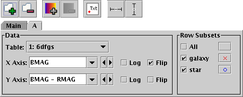
Default dataset selector from 2d scatter plot window
The different parts of this control work as follows:
The Axis selectors (here X Axis and Y Axis) give the quantities to be plotted. If you click the little down arrow at the right of each selector you get a list of all the numeric columns in the chosen table, from which you can select one. If you click the little left and right arrows to the right of the selector it will cycle through all the columns in the table. However, if you prefer you can type in an expression to use here. This may be more convenient if there's a very long list of columns (another way to deal with this is to hide most of the columns using the Column Window). However, what you type in doesn't have to be a column name, it can be an algebraic expression based on columns in the table, or even a constant. In the example, the X axis is a straight column name, and the Y axis is an expression. The expression language syntax is explained in Section 7.
The Log checkbox for each axis is used to select whether the scale should be logarithmic or linear.
The Flip checkbox for each axis is used to select whether the axis values increase in the conventional direction (left to right, bottom to top) or its opposite.
Some of the buttons in the toolbar shown will modify what is visible in this panel, for instance inserting new selectors to allow selection of error values. All the selectors work in the same way however.
The buttons to the right of each subset name show the symbol that is used in the plot to display the data from that subset, in this case a red cross and a blue circle. These are selected automatically when the subset is first selected for viewing (the initial default style set depends mainly on how many rows there are in the selected table - many rows gives small dots, few gives big ones). However, you have a lot of freedom to configure how they appear. If you click the button with the symbol on it a dialogue will pop up which allows you to select colour, shape, transparency and so on, as well as error bar style if appropriate and things like whether fitted lines will be plotted for that subset. The options available differ according to the kind of plot, and are described along with the different graphics windows in the following subsections. The style window stays visible until you dismiss it, but if you click on another of the buttons in the Row Subsets panel its contents will change to allow you to select values for the corresponding subset. Most graphics windows have a Marker Style menu. This allows you to change all the styles in the plot at once to be members of a uniform set, for instance different coloured pixels, or black open shapes. If you select one of these it will overwrite the existing style selections, but they can be edited individually afterwards.
The Add Dataset ( )
and Remove Dataset (
)
and Remove Dataset ( )
buttons in the toolbar add a new tab or remove the selected one
respectively.
Initially only the Main tab is present, and this one cannot be removed.
)
buttons in the toolbar add a new tab or remove the selected one
respectively.
Initially only the Main tab is present, and this one cannot be removed.
Sometimes (high-dimensional plots, auxiliary axes, error bars) a lot of information needs to be entered into the data panel, and the bottom part of the window can get quite large. Normally, the plot in the upper part of the window shrinks to accommodate it. You can of course resize the window to gain more space, but if your screen is small you may still end up with an uncomfortably small plot. If this happens, you can use the following button from the main toolbar:
 Split Window
In general terms the axes on which the graphics are plotted are defined by the datasets you have selected. The axis labels are set from the column names or expressions chosen for the Main dataset, and the ranges are determined so that all the data from the chosen datasets can be seen. However, these things can be adjusted manually.
The following features are available directly from the window for configuring axis range:
An easier alternative for zooming in the 3D windows is to use the mouse wheel, if you have one: wheel forward to zoom in and backward to zoom out.
Rescale
For more control over axis range and labelling, use the
Configure Axes and Title ( ) toolbar button,
which will pop up a dialogue like the following:
) toolbar button,
which will pop up a dialogue like the following:
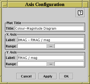
Axis Configuration Dialogue for 2-d axes
You can fill in these values for each axis as follows:
The plot title may also be set in the Plot Title panel of this window:
TOPCAT provides quite flexible graphical representation of symmetric or asymmetric errors in 1, 2 and 3 dimensions. The plots with error bar support are the 2D, 3D and spherical scatter plots and the stacked lines plot.
By default, error bar drawing is switched off. The simplest way to activate it is to use the relevant error bar button(s) in the data selector tool bar (the one below the plot). For the Cartesian (2D, 3D, lines) plots, some or all of the following buttons are present:
 X symmetric errors
 Y symmetric errors
 Z symmetric errors
Here is a 2D plot in which symmetric X and asymmetric Y errors are being used:
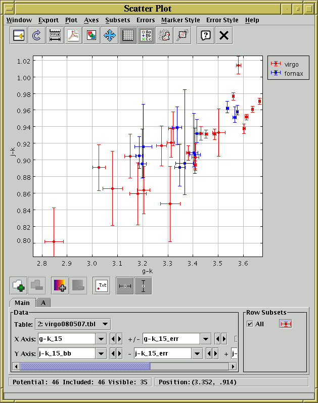
Plot window with symmetric X and asymmetric Y errors
You can see that with the error column selector, the panel has become too wide for the window so a scrollbar has appeared at the bottom - you can scroll this left and right or enlarge the window to see the parts that you need to.
For the spherical plot the following error toggle buttons are present:
 tangential isotropic errors
radial symmetric errors
tangential isotropic errors
radial symmetric errors
If you want to use asymmetric or one-sided errors, use the options in the Errors menu instead of the toolbar buttons. For instance the options for X axis error bars in the 2D scatter plot are:
 None
None
 Symmetric
 Lower Only
 Upper Only
 Lower & Upper
There are many options for the plotting style of one, two and three dimensional error bars, including capped and uncapped bars, crosshairs, ellipses and rectangles. This plotting style is controlled from the plot window's Style Editor window (see e.g. Appendix A.5.3.1), which can be viewed by clicking on the marker icon in the Row Subsets panel at the bottom right of the window. The available error bar styles will depend on which axes currently have errors; if none do, then the error bar selector will be disabled. You can also use the Error Style menu to change the error style for all the visible datasets at once.
On the 2-d and 3-d scatter plots you can write text labels adjacent
to plotted points. To do this click the Draw Labels
( ) button in the dataset toolbar (below the plotting area
in the plot window). This will reveal a new Point Labels
selector below the existing spatial ones.
Using this you can select any of the table columns (not just the
numeric ones as for the other selectors), or give a string or
numeric expression involving them. When this selector is filled
in, every point in the dataset which has a non-blank value for
this quantity will have it written next to the point on the display.
) button in the dataset toolbar (below the plotting area
in the plot window). This will reveal a new Point Labels
selector below the existing spatial ones.
Using this you can select any of the table columns (not just the
numeric ones as for the other selectors), or give a string or
numeric expression involving them. When this selector is filled
in, every point in the dataset which has a non-blank value for
this quantity will have it written next to the point on the display.
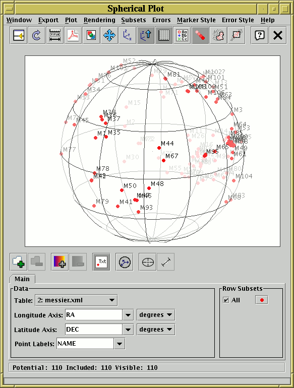
Point Labelling for Messier objects in the spherical plot
In this example the NAME column has been selected, so that each point plotted (in this case all the Messier objects) is labelled with its name. As you can see, where many labels are plotted near to each other they can get in each others' way. In some cases TOPCAT will omit plotting labels in crowded regions, in others not - but in any case if you have labels too tightly grouped they are unlikely to be legible.
TOPCAT can plot data in one, two or three spatial dimensions, but sometimes the the data which you need to visualise is of higher dimensionality. For this purpose, some of the plotting windows (2D and 3D scatter plots) allow you to control the colouring of plotted points according to values from one or more additional columns (or calculated expressions), which gives you more visual information about the data you are examining.
To use this facility, click the Add auxiliary axis
( ) button in the dataset toolbar (below the plot area
in a plot window).
A new axis selector will appear below the existing spatial ones,
labelled Aux 1 Axis. It has log and flip checkboxes
like the spatial axes, and to the right (you may need to widen the
window or use the scrollbar at the bottom to see it) is a selector depicting a
number of colourmaps to choose from - the default one resembling a
rainbow is usually quite suitable, but you can pick others.
If you enter a column name or expression into the selector, each
plotted point will be coloured according to the value of that quantity
in the corresponding row of data. If that quantity is null for a row,
the corresponding point will not be plotted.
A scale on the right of the plot indicates how the colour map
corresponds to numeric values.
To remove the auxiliary axis and go back to normally-coloured points,
simply click the Remove auxiliary axis (
) button in the dataset toolbar (below the plot area
in a plot window).
A new axis selector will appear below the existing spatial ones,
labelled Aux 1 Axis. It has log and flip checkboxes
like the spatial axes, and to the right (you may need to widen the
window or use the scrollbar at the bottom to see it) is a selector depicting a
number of colourmaps to choose from - the default one resembling a
rainbow is usually quite suitable, but you can pick others.
If you enter a column name or expression into the selector, each
plotted point will be coloured according to the value of that quantity
in the corresponding row of data. If that quantity is null for a row,
the corresponding point will not be plotted.
A scale on the right of the plot indicates how the colour map
corresponds to numeric values.
To remove the auxiliary axis and go back to normally-coloured points,
simply click the Remove auxiliary axis ( )
button.
)
button.
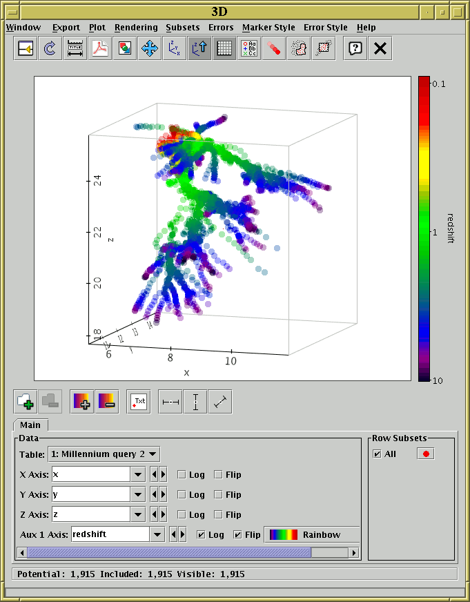
3D plot of simulation data showing X, Y, Z spatial position with the auxiliary axis indicating timestep.
There are two types of colour maps you can choose from: colour fixing and colour modifying. The fixing ones are easiest to understand: the original colour of the point (as drawn in the legend) is ignored, and it is coloured according to the relevant value on the selected auxiliary axis. The colour modifying maps take the original colour and affect it somehow, for instance by changing its transparency or its blue component. These are marked with an asterisk ("*") in the colour map selector. They can be used to convey more information but are often harder to interpret visually - for one thing the shading of the colour bar in the legend will not correspond exactly to the colours of the plotted points.
By using modifying colour maps it is possible to perform plots with more than one auxiliary axis - typically the first one will be a fixing map and subsequent ones will be modifying. So the first auxiliary axis could have the (fixing) Rainbow map, and the second could have the (modifying) Transparency map. The colour alterations are applied in order. It is possible, but pointless, to have multiple fixing maps applied to the same points - the last-numbered one will determine the colour and earlier ones will get ignored. Multiple aux axes can be obtained by clicking the Add auxiliary axis button more than once. When combining several maps some thought has to be given to which ones to use - some good combinations are the three RGB ones or the three YUV ones.
A fairly wide range of colour maps of both kinds is provided by default. If these do not suit your needs, it is possible to provide your own custom colour fixing maps using the lut.files system property - see Section 10.2.3.
It is easy to generate attractive screenshots using auxiliary axes. Making visual sense of the results is a different matter. One visualisation expert tried to dissuade their introduction in TOPCAT on the grounds that the graphics they produce are too hard for humans to interpret - I hope that these plots can assist with some analysis, but it is a somewhat experimental feature which may or may not end up being widely useful. The maximum number of auxiliary axes which can be used together is currently three. This could be increased on request, but if you feel you can generate an intelligible plot using more than this then you're considerably smarter than me.
When quantities are plotted in one of the graphics windows it becomes easy to see groupings of the data which might not otherwise be apparent; a cluster of (X,Y) points representing a group of rows may correspond to a physically meaningful grouping of objects which you would like to treat separately elsewhere in the program, for instance by calculating statistics on just these rows, writing them out to a new table, or plotting them in a different colour on graphs with different coordinates. This is easily accomplished by creating a new Row Subset containing the grouped points, and the graphics windows provide ways of doing this.
In some of the plots
(Histogram
2d Scatter plot
Density map and
Spherical plot)
you can set the axis ranges (either manually or by zooming with the
mouse - see Appendix A.5.1.2)
so that only the points you want to identify are visible,
and then click the
Subset From Visible toolbar button
(the icon is ,  or
or  depending on the plot type).
This defines a subset consisting of all the
points that are visible on the current plot.
This is only useful if the group you are interested in
corresponds to a rectangular region in the plotting space.
depending on the plot type).
This defines a subset consisting of all the
points that are visible on the current plot.
This is only useful if the group you are interested in
corresponds to a rectangular region in the plotting space.
A more flexible way is to draw a region or regions
on the plot which identify the points you are interested in.
To do this, hit the
Draw Subset Region ()
toolbar button. Having done this, you can drag the mouse around
on the plot (keep the left mouse button down while you move)
to encircle the points that you're interested in.
As you do so, a translucent grey blob will be left behind -
anything inside the
blob will end up in the subset. You can draw one or many blobs,
which may be overlapping or not. If you make a mistake while
drawing a sequence of blobs, you can click the right mouse button,
and the most recently added blob will disappear.
When you're in this region-drawing mode,
you can't zoom or resize the window or change the characteristics
of the plot, and the Draw Subset Region button
appears with a tick over it () to remind you
you're in it. Here's what the plot looks like while you're drawing:
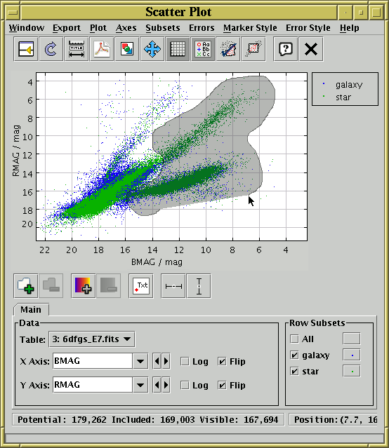
Region-Drawing Mode
When you're happy with the region you've defined, click the
toolbar button again.
In either case, when you have indicated that you want to define a new row subset, a dialogue box will pop up to ask you its name. As described in Section 3.1.1, it's a good idea to use a name which is just composed of letters, numbers and underscores. You can optionally select a subset name which has been used before from the list, which will overwrite the former contents of that subset. When you enter a name and hit the OK button, the new subset will be created and the points in it will be shown straight away on the plot using a new symbol. As usual, you can toggle whether the points in this subset are displayed using the Row Subsets box at the bottom of the Plot Window.
All the old-style graphics windows have the following export options in the toolbar:
 Export as PDF
Export as GIF
Export as PDF
Export as GIF
 Export as Encapsulated PostScript
 Export as Gzipped Encapsulated PostScript
 Export as JPEG
Export as PNG
Export as JPEG
Export as PNG
Exporting to the pixel-based formats (GIF, JPEG, PNG) is fairly straightforward: each pixel on the screen appears as one pixel in the output file. PNG is the most capable, but it is not supported by all image viewers. GIF works well in most cases, but if there are more than 255 colours some of the colour resolution will be lost. JPEG can preserve a wide range of colours, but does not support transparency and is lossy, so close inspection of image features will reveal blurring.
When exporting to Portable Document Format (PDF), Scalable Vector Graphics (SVG) or Encapsulated PostScript (EPS), which are vector graphics formats, there are a few things to consider:
This section describes an old-style plotting window. The standard plotting windows are described in Appendix A.4.
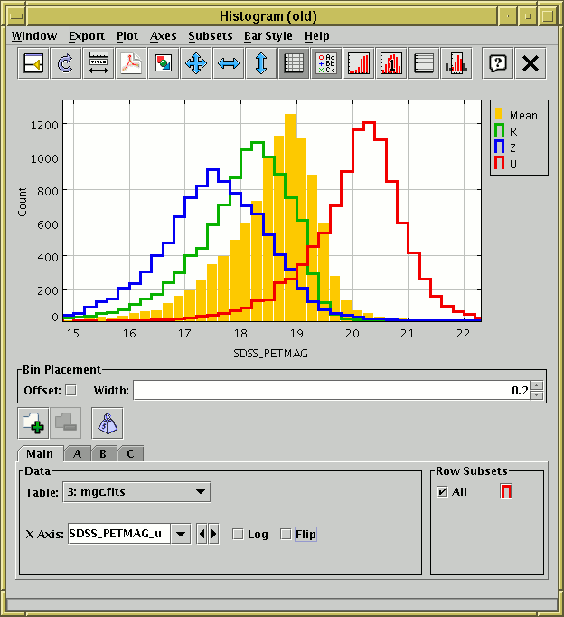
Histogram Window
The histogram window lets you plot histograms of one or more
columns or derived quantities.
You can display it using the Histogram ()
item in the Control Window's
Graphics menu.
You select the quantity or quantities to plot using the dataset selector at the bottom of the window. You can configure the axes, including zooming in and out, with the mouse (drag on the plot or the axes) or manually as described in Appendix A.5.1.2.
The Bin Placement box below the main plot controls where the bars are drawn. Select the horizontal range of each bar using the Width entry box - either type in the value you want or use the tiny up/down arrows at the right to increase/decrease the bin size. The Offset checkbox on the left determines where the zero point on the horizontal axis falls in relation to the bins; if the box is checked then zero (or one for logarithmic X axis) is in the centre of a bin, and if it's unchecked then zero (or one) is on a bin boundary.
The following buttons are available on the toolbar:
Split Window
Replot
Configure Axes and Title
Export as PDF
Export as GIF
Rescale
 Grid
Show Legend
Grid
Show Legend
 Cumulative Plot
 Normalisation
 Log Y Axis
Subset From Visible
Log Y Axis
Subset From Visible
The Dataset Toolbar contains the following options:
/ Add/Remove dataset
 Weight Counts
When weighted, bars can be of negative height. An anomaly of the plot as currently implemented is that the Y axis never descends below zero, so any such bars are currently invisible. This may be amended in a future release (contact the author to vote for such an amendment).
The Export menu contains additional image export options and the following options specific to the histogram:
Save as Table
Import as Table
You have considerable freedom to configure how the bars are drawn; controlling this is described in the following subsection.
The bins in a histogram can be represented in many different ways. A representation of how a bar will be displayed is shown on a button to the right of the name of each visible subset, at the bottom right of the histogram window. If you click this button the following dialogue will pop up which enables you to change the appearance.
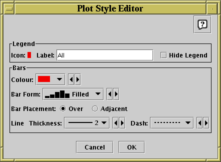
Style editor dialogue for histogram bars
The Legend box defines how the selected set will
be identified in the legend which appears alongside the plot
(though the legend will only be visible if Show Legend
() is on):
The Bins panel describes the form of the bars to be plotted for each data set.
Any changes you make in this window are reflected in the plot straight away. If you click the OK button at the bottom, the window will disappear and the changes remain. If you click Cancel the window will disappear and any changes you made will be discarded.
You can also change all the plotting styles at once by using the Bar Style menu in the histogram window. Here you can select a standard group of styles (e.g. all filled adjacent bars with different colours) for the plotted sets.
This section describes an old-style plotting window. The standard plotting windows are described in Appendix A.4.
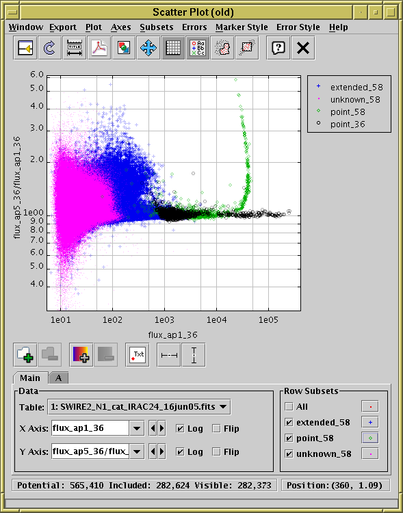
Plot Window
The plot window allows you to do 2-dimensional scatter plots of
one or more pair of table columns (or derived quantities).
You can display it using the Plot () item
in the Control Window's
Graphics menu.
On the plotting surface a marker is plotted for each row in the selected dataset(s) at a position determined by the values in the table columns selected to provide the X and Y values. A marker will only be plotted if both the X and Y values are not blank. Select the quantities to plot and the plotting symbols with the dataset selector at the bottom. You can configure the axes, including zooming in and out, with the mouse (drag on the plot or the axes) or manually as described in Appendix A.5.1.2.
Clicking on any of the plotted points will activate it - see Section 8.
The following buttons are available on the toolbar:
Split Window
Replot
Configure Axes and Title
Export as PDF
Export as GIF
Rescale
Grid
Show Legend
Draw Subset Region
Subset From Visible
The Dataset Toolbar contains the following options:
/ Add/Remove dataset
/ Add/Remove auxiliary axis
Toggle point labelling
/ Toggle X/Y error bars
You have considerable freedom to configure how the points are plotted including the shape, colour and transparency of symbols, the type of lines which join them if any, and the representation of error bars if active. These options are described in the following subsection.
When plotting points in a scatter plot there are many different ways that each point can be displayed. By default, TOPCAT chooses a set of markers on the basis of how many points there are in the table and uses a different one for each plotted set. The marker for each set is displayed in a button to the right of its name in the dataset selector panel at the bottom of the plot window. If you click this button the following dialogue will pop up which enables you to change the appearance.
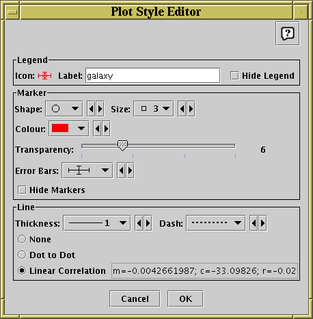
Style editor dialogue for 2d scatter plot
The Legend box defines how the selected set will
be identified in the legend which appears alongside the plot
(though the legend will only be visible if Show Legend
() is on):
The Marker box defines how the markers plotted for each data point will appear:
The Line box determines if any lines are drawn associated with the current set and if so what their appearance will be.
Note that for both the plotted line and the quoted coefficients the data is taken only from the points which are currently visible - that means that if you've zoomed the axes to exclude some of the data points, they will not be contributing to the calculated statistics.
Any changes you make in this window are reflected in the plot straight away. If you click the OK button at the bottom, the window will disappear and the changes remain. If you click Cancel the window will disappear and any changes you made will be discarded.
You can also change all the plotting styles at once by using the Marker Style menu in the plot window. Here you can select a standard group of styles (e.g. all open 2-pixel markers with different colours and shapes) for the plotted sets. Similarly, error styles can be changed all at once using the Error Style menu.
This section describes an old-style plotting window. The standard plotting windows are described in Appendix A.4, though note that at time of writing (v4.1) no equivalent new-style plotting window is available for plotting stacked lines.
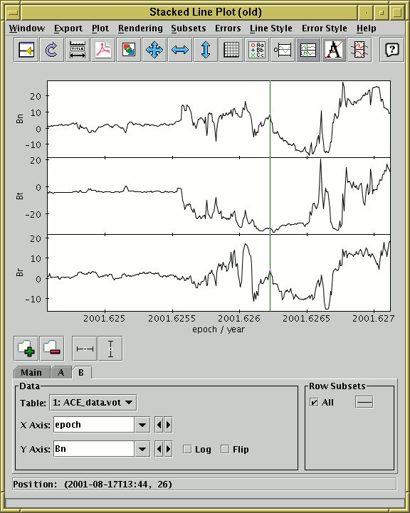
Stacked Lines Window
The stacked line plot window allows you to plot one or more ordinate (Y)
quantities against a monotonic abscissa (X) quantity.
For clarity, the different plots are displayed on vertically
displaced graphs which share the same X axis.
You can display this window using the Lines ()
item in the Control Window's
Graphics menu.
The display initially holds a single X-Y graph, usually with lines connecting adjacent points. The points will be reordered before drawing if necessary so that the line is displayed as a function of X, rather than of an invisible third independent variable (in the Scatter Plot this isn't done which can lead to lines being scribbled all over the plot). If one of the columns in the table appears to represent a time value, this will be selected as the default X axis. Otherwise, the 'magic' index variable will be used, which represents the row number. Of course, these can be changed from their default values using the selectors in the usual way.
To add a new graph with a different Y axis, use the
Add Dataset () button in the
Dataset Toolbar at the bottom of the window.
This has a slightly different effect from what it does in the other
plot windows, in that it inserts a new plotting region with its own
Y axis at the top of the plot on which the specified data is drawn,
rather than only causing a new set of points to be plotted on the
existing plot region.
Thus all the datasets appear in their own graphs with their own Y axes
(though if you have multiple row subsets plotted for the same
dataset they will appear on the same part of the plot as usual).
To remove one of the graphs, select its tab and use the
Remove Dataset () button as usual.
Zooming can only be done on one axis at a time
rather than dragging out an X-Y region on the plot surface, since
there isn't a single Y axis to zoom on.
To zoom the X axis in/out, position the mouse just below the X axis
at the bottom of the plot and drag right/left.
To zoom one of the Y axes in or out, position the mouse just to the
left of the Y axis you're interested in and drag down/up.
To set the ranges manually, use the Configure Axes and Title
() button as usual, but note that there is one
label/range setting box for each of the Y axes.
These things work largely as described in Appendix A.5.1.2,
as long as you bear in mind that the range of each of the Y axes
is treated independently of the others.
Clicking on any of the points will activate it - see Section 8.
The following buttons are available on the toolbar:
Split Window
Configure Axes and Title
Export as PDF
Export as GIF
Rescale
Full Grid
Show Legend
 y=0 Grid Lines
 Show Vertical Crosshair
 Antialias
Subset From X Range
Antialias
Subset From X Range
The Dataset Toolbar contains the following options:
/ Add/Remove dataset
/ Toggle X/Y error bars
You can determine how the data are plotted using lines and/or markers as described in the following subsection.
The default plotting style for the stacked lines plot is a simple black line for each graph. Since the plots typically do not overlap each other, this is in many cases suitable as it stands. However, you can configure the plotting style so that the points are plotted with markers as well as or instead of lines, and change the colours, marker shapes, line styles etc. The style for each row subset is displayed in a button to the right of its name in the bottom right of the plotting window. If you click this button the following dialogue will pop up which entables you to configure the plotting style.
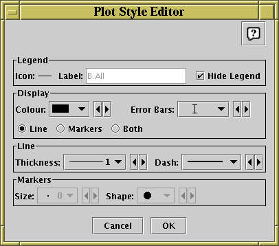
Stacked Line Plot Style Editor
The Legend box defines how the selected set will
be identified in the legend which appears alongside the plot
(though the legend will only be visible if Show Legend
() is on):
The Display box defines how the markers plotted for each data point will appear:
The Line box defines how the lines joining the points will look. These controls will only be active if the Display selection is Line or Both.
The Markers box defines how markers at the data points will look. These controls will only be active if the Display selection is Markers or Both.
Any changes you make in this window are reflected in the plot straight away. If you click the OK button at the bottom, the window will disappear and the changes remain. If you click Cancel the window will disappear and any changes you made will be discarded.
You can also change all the plotting styles at once by using the Line Style menu in the stacked lines plot window. Here you can select a standard group of styles (e.g. dashed lines, coloured lines) for the plotted sets. Similarly, error styles can be changed all at once using the Error Style menu.
This section describes an old-style plotting window. The standard plotting windows are described in Appendix A.4.
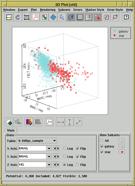
3D scatter plot window
The 3D plot window draws 3-dimensional scatter plots of one or more
triples of table columns (or derived quantities) on Cartesian axes.
You can display it using the 3D () item
in the Control Window's
Graphics menu.
On the display a marker is plotted for each row in the selected dataset(s) at a position determined by the values in the table columns selected to provide the X, Y and Z values. A marker will only be plotted if none of the X, Y and Z values are blank. Select the quantities to plot and the plotting symbols with the dataset selector at the bottom.
The 3D space can be rotated by dragging the mouse around on the surface - it will rotate around the point in the centre of the plotted cube. The axis labels try to display themselves the right way up and in a way which is readable from the viewing point if possible, which means they move around while the rotation is happening. By default the points are rendered as though the 3D space is filled with a 'fog', so that more distant points appear more washed out - this provides a visual cue which can help to distinguish the depth of plotted points. However, you can turn this off if you want. If there are many points, then you may find that they're not all plotted while a drag-to-rotate gesture is in progress. This is done to cut down on rendering time so that GUI response stays fast. When the drag is finished (i.e. when you release the mouse button) all the points will come back again.
Zooming is also possible. You can zoom in around the
centre of the plot so that the viewing window only covers the middle.
The easiest way to do this is to use the mouse wheel if you have one -
wheel forward to zoom in and backward to zoom out.
Alternatively you can do it by dragging on the region to the left of
the plot, like the Axis Zoom in some of the 2-d plots.
Drag the mouse down to zoom in or up to zoom
out on this part of the window. Currently it is only possible
to zoom in/out around the centre of the plot.
When zoomed you can use the
Subset From Visible () toolbar button
to define a new Row Subset consisting only of the
points which are currently visible.
See Appendix A.5.1.6 for more explanation.
Clicking on any of the plotted points will activate it - see Section 8.
The following buttons are available on the toolbar:
Split Window
Replot
Configure Axes and Title
Export as PDF
Export as GIF
Rescale
 Reorient
 Stay Upright
Grid
Show Legend
Stay Upright
Grid
Show Legend
 Fog
Draw Subset Region
Subset From Visible
Fog
Draw Subset Region
Subset From Visible
The following additional item is available as a menu item only:
Antialias
The Dataset Toolbar contains the following options:
/ Add/Remove dataset
/ Add/Remove auxiliary axis
Toggle point labelling
/ / Toggle X/Y/Z error bars
You have considerable freedom to configure how the points are plotted including the shape, colour and transparency of symbols and the representation of error bars if used. These options are described in the following subsection.
When plotting points in a 3D plot there are many different ways that each point can be displayed. By default, TOPCAT chooses a set of markers on the basis of how many points there are in the table and uses a different one for each plotted set. The marker for each set is displayed in a button to the right of its name in the dataset selector panel at the bottom of the plot window. If you click this button the following dialogue will pop up which enables you to change the appearance.
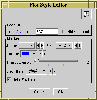
Style editor dialogue for 3d plots
The Legend box defines how the selected set will
be identified in the legend which appears alongside the plot
(though the legend will only be visible if Show Legend
() is on):
The Marker box defines how the markers plotted for each data point will appear:
Any changes you make in this window are reflected in the plot straight away. If you click the OK button at the bottom, the window will disappear and the changes remain. If you click Cancel the window will disappear and any changes you made will be discarded.
You can also change all the plotting styles at once by using the Marker Style menu in the plot window. Here you can select a standard group of styles (e.g. all open 2-pixel markers with different colours and shapes) for the plotted sets. Similarly, error styles can be changed all at once using the Error Style menu.
This section describes an old-style plotting window. The standard plotting windows are described in Appendix A.4.
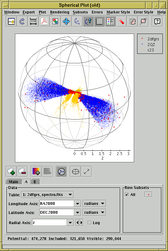
Spherical plot window
The spherical plot window draws 3-dimensional scatter plots
of datasets from one or more tables on spherical polar axes,
so it's suitable for displaying the position of coordinates on
the sky or some other spherical coordinate system, such as the
surface of a planet or the sun.
You can display it using the Sphere () item
in the Control Window's
Graphics menu.
In most respects this window works like the 3D Plot window, but it uses spherical polar axes rather than Cartesian ones, You have to fill in the dataset selector at the bottom with longitude- and latitude-type coordinates from the table. Selectors are included to indicate the units of those coordinates. If TOPCAT can locate columns in the table which appear to represent Right Ascension and Declination, these will be filled in automatically. If only these two are filled in, then the points will be plotted on the surface of the unit sphere - this is suitable if you just want to inspect the positions of a set of objects in the sky.
If the Radial Coordinates ( ) button is
activated, you can optionally fill in a value in the
Radial Axis selector as well.
In this case points will be plotted in the interior of the sphere,
at a distance from the centre given by the value of the radial coordinate.
) button is
activated, you can optionally fill in a value in the
Radial Axis selector as well.
In this case points will be plotted in the interior of the sphere,
at a distance from the centre given by the value of the radial coordinate.
The 3D space can be rotated by dragging the mouse around on the surface - it will rotate around the centre of the sphere. By default the points are rendered as though the 3D space is filled with a 'fog', so that more distant points appear more washed out - this provides a visual cue which can help to distinguish the depth of plotted points. However, you can turn this off if you want. If there are many points, then you may find that they're not all plotted while a drag-to-rotate gesture is in progress. This is done to cut down on rendering time so that GUI response stays fast. When the drag is finished (i.e. when you release the mouse button) all the points will come back again.
Zooming is also possible. You can zoom in around the
centre of the plot so that the viewing window only covers the middle.
The easiest way to do this is to use the mouse wheel if you have one -
wheel forward to zoom in and backward to zoom out.
Alternatively you can do it by dragging on the region to the left of
the plot, like the Axis Zoom in some of the 2-d plots.
Drag the mouse down to zoom in or up to zoom
out on this part of the window. Currently it is only possible
to zoom in/out around the centre of the plot.
When zoomed you can use the
Subset From Visible () toolbar button
to define a new Row Subset consisting only of the
points which are currently visible.
See Appendix A.5.1.6 for more explanation.
Clicking on any of the plotted points will activate it - see Section 8.
The following buttons are available on the toolbar:
Split Window
Replot
Configure Axes and Title
Export as PDF
Export as GIF
Rescale
Reorient
Stay Upright
Grid
Show Legend
Fog
Draw Subset Region
Subset From Visible
The following additional item is available as a menu item only:
Antialias
The Dataset Toolbar contains the following options:
/ Add/Remove dataset
/ Add/Remove auxiliary axis
Toggle point labelling
Toggle Radial Coordinates
Toggle tangential error bars
Toggle radial error bars
You have considerable freedom to configure how points are plotted including the shape, colour and transparency of symbols and the representation of errors if used. This works exactly as for the Cartesian 3D plot as described in Appendix A.5.5.1.
This section describes an old-style plotting window. The standard plotting windows are described in Appendix A.4.
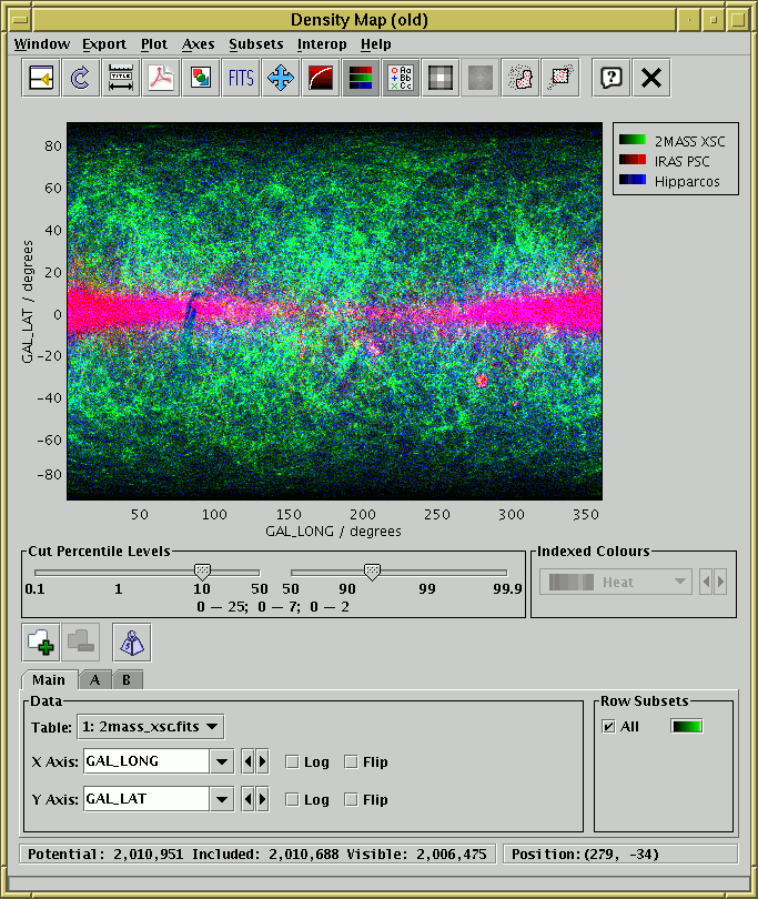
Density map window in RGB mode
The density map window plots a 2-dimensional density map of one or more pairs of table columns (or derived quantities); the colour of each pixel displayed is determined by the number of points in the data set which fall within its bounds. Another way to think of this is as a histogram on a 2-dimensional grid, rather than a 1-dimensional one as in the Histogram Window. You can optionally weight these binned counts with another value from the table.
Density maps are suitable when you have a very large number of points to plot, since in this case it's important to be able to see not just whether there is a point at a given pixel, but how many points fall on that pixel. To a large extent, the transparency features of the other 2d and 3d plotting windows address this issue, but the density map gives you a bit more control. It can also export the result as a FITS image, which can then be processed or viewed using image-specific software such as GAIA or Aladin.
This window can be operated in two modes:
 ) button.
You can configure the axes, including zooming in and out, with the mouse (drag on the plot or the axes) or manually as described in Appendix A.5.1.2.
Two controls specific to this window are shown below the plot itself:
The following buttons are available on the toolbar:
Split Window
Replot
Configure Axes and Title
Export as PDF
Export as GIF
 Export as FITS
Rescale
Export as FITS
Rescale
 Log Intensity
Colour
Show Legend
Log Intensity
Colour
Show Legend
 Bigger Pixels
 Smaller Pixels
Draw Subset Region
Subset From Visible
Smaller Pixels
Draw Subset Region
Subset From Visible
The Dataset Toolbar contains the following options:
/ Add/Remove dataset
Weight Counts
The Export menu provides a number of ways to export the displayed image for external viewing or analysis. As well as options to export as GIF, JPEG, EPS and FITS, there is also the option to transmit the FITS image to one or all applications listening using the SAMP or PLASTIC tool interoperability protocol which will receive images. In this way you can transmit the image directly to SAMP/PLASTIC-aware image manipulation tools such as GAIA or Aladin. See Section 9 for more information about tool interoperability.
How to set the colour channel corresponding to each dataset is explained in the following subsection.
For a density map in RGB mode, each dataset is assigned a colour channel to which it contributes. A representation of this is displayed in a button to the right of its name in the dataset selector panel at the bottom of the density map window. If you click this button the following dialogue will pop up which enables you to change the colour channel.
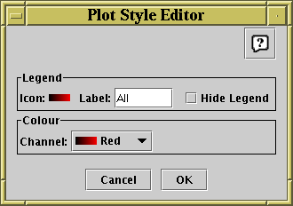
Style editor dialogue for density map
The Legend box defines how the selected set will
be identified in the legend which appears alongside the plot
(though the legend will only be visible if Show Legend
() is on):
The Channel selector allows you to select either the Red, Green or Blue channel for this dataset to contribute to. Note that this is only enabled in RGB mode; in indexed mode it has no effect and is disabled.
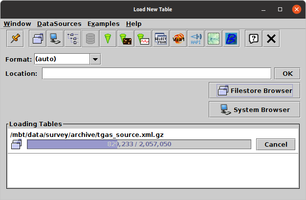
Load Window
The Load Window is used for loading tables from an external location
(e.g. disk or URL) into TOPCAT. It is obtained using the
Load Table button () in the
Control Window toolbar or
File menu.
This dialogue allows you to specify a new table to open in a number of different ways, described below. If you perform a successful load using any of these options, a new entry or entries will be added into the Table List in the Control Window, which you can then use in the usual ways. If you choose a location which can't be turned into a table (for instance because the file doesn't exist), a window will pop up telling you what went wrong. The panel at the bottom of the window displays progress for tables currently loading; it is used to show progress for tables loaded from other sources too, for instance received via SAMP or specified on the command line.
In the simplest case, you can type a name into the
Location field and hit return or the OK
button. This location can be a filename or a URL,
possibly followed by a '#' character and a
'fragment identifier' to indicate where in the file or URL the table is
located; the details of what such fragment identifiers mean can be
found in the relevant subsection within Section 4.1.1.
Allowed URL types are described in Section 4.2.
You should select the relevant table format from the
Format selector box - in many cases
(file formats that can be recognised by content such as
FITS or VOTable, or files named in a conventional way
such as CSV files with the ".csv" extension)
the default (auto) setting will work,
but in other cases TOPCAT may not be able to guess the file format,
and you have to select the right one explicitly
(again, see Section 4.1.1 for details).
You can also enter a
scheme specification
into the Location field.
These have the form ":<scheme-name>:<scheme-args>"
and can be used for tables that are created in some other way
than reading a stream of bytes;
for instance ":skysim:1e6" generates a simulated
sky survey with a million rows.
There are many other ways of loading tables however, described in the following subsections. The Filestore Browser and System Browser buttons are always visible below the location field. Depending on startup options, there may be other buttons here. There are also a number of toolbar buttons which display various load dialogues; the DataSources contains all of these along with some lesser-used ones. The following subsections describe most of the available options, though others may be available in your installation.
The options available on the toolbar by default are these:
 Filestore Browser
 System Browser
 Hierarchy Browser
 SQL Query
 Cone Search
 Simple Image Access (SIA) Query
 Simple Spectral Access (SSA) Query
Table Access Protocol (TAP) Query
Simple Spectral Access (SSA) Query
Table Access Protocol (TAP) Query
 VizieR Catalogue Service Query
 HAPI query
 Virgo-Millennium Simulation Query
All of these load dialogues have an OK button. Once you click it, whatever load you have specified will start. If the load takes more than a few hundreths of a second, a progress bar will appear in the Loading Tables panel of the load window, as in the screenshot above. This will report on how many rows have been loaded, and if known, how many there are in total. If you want to interrupt the load for any reason while it is in progress, click the Cancel button, and the load will cease. If the load completes without cancellation, a new table will appear in the Table List of the main Control Window, ready for use.
By default, when a table load has completed, both the Load Window
itself and whichever specific load dialogue window you used will close.
If you don't want this to happen use the
Stay Open ( ) item
in the Window menu or
toolbar of the Load Window and/or specific load dialogue.
If this is selected, the window will not automatically close.
This can be very convenient if you want to load many tables from
a similar place, for instance several files from the same directory
or several cone searches to different services.
) item
in the Window menu or
toolbar of the Load Window and/or specific load dialogue.
If this is selected, the window will not automatically close.
This can be very convenient if you want to load many tables from
a similar place, for instance several files from the same directory
or several cone searches to different services.
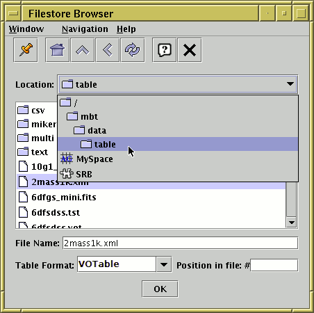
Filestore Browser window
By clicking the Filestore Browser button
or toolbar button () in the
Load Window,
you can obtain a file browser which will
display the files in a given directory.
The way this window works is almost certainly familiar to you
from other applications.
Unlike a standard file browser however, it can also browse files in remote filestores: currently supported are MySpace and SRB. MySpace is a distributed storage system developed for use with the Virtual Observatory by the AstroGrid project, and SRB (Storage Resource Broker) is a similar general purpose system developed at SDSC. To make use of these facilities, select the relevant entry from the selector box at the top of the window as illustrated above; this will show you a Log In button which prompts you for username, password etc, and you will then be able to browse the remote filestore as if it were local. The same button can be used to log out when you are finished, but the session will be logged out automatically when TOPCAT ends in any case.
The browser initially displays the current directory, but this can be
changed by typing a new directory into the File Name field,
or moving up the directory hierarchy using the selector box at the top,
or navigating the file system by clicking the up-directory button
or double-clicking on displayed directories.
The initial default directory can be changed by setting the
user.dir
system property.
All files are shown, and there is no indication of which ones represent tables and which do not. To open one of the displayed files as a table, double-click on it or select it by clicking once and click the Open Table button. The Table Format selector must be set correctly: the "(auto)" setting will automatically detect the format of VOTable or FITS tables, otherwise you will need to select the option describing the format of the file you are attempting to load (see Section 4.1.1). If you pick a file which cannot be converted into a table an error window will pop up.
In most cases, selecting the file name and possibly the format is all you need to do. However, the Position in file field allows you to add information about where in the file the table you want is situated. The meaning of this varies according to the file format: for FITS files, it is the index or EXTNAME of the HDU containing the table you're after (see Section 4.1.1.1 for details), and for VOTables it is the index of the TABLE element (the first TABLE encountered is numbered 0). If you leave this blank, you will get all the tables in the file; this is usually just one table, since most file formats cannot accommodate more than one table per file, and even for those which can (FITS and VOTable) most files contain only a single file in any case.
For a more table-aware view of the file system, use the Hierarchy Browser instead.
By clicking the System Browser button or toolbar button
() in the
Load Window,
you can use your Operating System's native file browser to choose
a file to load from.
What this looks like is entirely dependent on your OS;
it may or may not contain system-specific features like shortcuts to
commonly-used directories.
Since TOPCAT has no control over the way this dialogue looks, it cannot contain the Table Format selector, and certain other things such as load cancel may not work as well as for the other dialogue types. To select the table format, you will need to use the selector in the main Load Window.
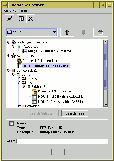
File load Hierarchy Browser window
By selecting the Hierarchy Browser button
()
from the Load Window's toolbar
or DataSources menu,
you can obtain a browser which presents a table-aware
hierarchical view of the file system.
(Note that a freestanding version of this panel with additional
functionality is available in the separate
Treeview
application).
This browser resembles the Filestore Browser in some ways, but with important differences:
The main part of the window shows a "tree" representation of the
hierarchy, initially rooted at the current directory
(the initial directory can be changed by setting the
user.dir
system property).
Each line displayed represents a "node" which may be a file or
some other type of item (for instance an HDU in a FITS file or an
entry in a tar archive). The line contains a little icon
which indicates what kind of node it is and a short text string which
gives its name and maybe some description.
Nodes which represent tables are indicated by the
icon.
For nodes which have some internal structure there is also a
"handle" which indicates whether they are
collapsed ( ) or expanded (
 ).
You can examine remote filespaces (MySpace, SRB)
as well as local ones in the same way as with the
Filestore Browser.
).
You can examine remote filespaces (MySpace, SRB)
as well as local ones in the same way as with the
Filestore Browser.
If you select a node by clicking on it, it will be highlighted and some additional description will appear in the panel below the hierarchy display. The text is in bold if the node in question can be opened as a table, and non-bold if it is some non-table item.
Note: an important restriction of this browser is that it will only pick up tables which can be identified automatically - this includes FITS and VOTable files, but does not include text-based formats such as ASCII and Comma-Separated Values. If you want to load one of the latter types of table, you will need to use one of the other load methods and specify table format explicitly.
You can see how this browser works on an example directory of tables as described in Appendix A.6.12.
Note that this window requires certain optional components of the TOPCAT installation, and may not always be available.
Navigation is a bit different from navigation in the File Browser window. To expand a node and see its contents, click on its handle (clicking on the handle when it is expanded will collapse it again). When you have identified the table you want to open, highlight it by clicking on it, and then click the Open Table button at the bottom.
To move to a different directory, i.e. to change the root of the tree which is displayed, use one of the buttons above the tree display:
 Up
Up
 Down
Down
 Home
Home
(In fact the above navigation options are not restricted to changing the root to a new directory, they can move to any node in the tree, for instance a level in a Tar archive.)
There are two more buttons in the browser, Search Selected and Search Tree. These do a recursive search for tables in all the nodes starting at the currently selected one or the current root respectively. What this means is that the program will investigate the whole hierarchy looking for any items which can be used as tables. If it finds any it will open up the tree so that they are visible (note that this doesn't mean that the only nodes revealed will be tables, ancestors and siblings will be revealed too). This can be useful if you believe there are a few tables buried somewhere in a deep directory structure or Tar archive, but you're not sure where. Note that this may be time-consuming - a busy cursor is displayed while the search is going on. Changing the root of the tree will interrupt the search.
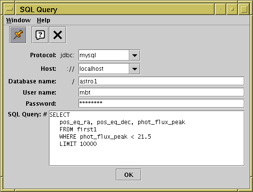
SQL Query Dialogue
If you want to read a table from an SQL database,
you can use a specialised dialogue to specify the SQL query by selecting
SQL Query button from the
Load Window's
toolbar () or DataSources menu.
This provides you with a list of fields to fill in which make up the query, as follows:
mysql" for MySQL's Connector/J driver
or "postgresql" for PostgreSQL's JDBC driver.
localhost" if the database is local).
SELECT * from XXX".
In principle any SQL query on the database can be used here,
but the details of what SQL syntax is permitted may be restricted
by the JDBC driver you are using.
There are a number of criteria which must be satisfied for SQL access to work within TOPCAT (installation of appropriate drivers and so on) - see Section 10.3. If you don't take these steps, this dialogue may be inaccessible.
The way that this dialogue contacts the database makes some assumptions about how the JDBC driver works which are not always true, so for some databases and drivers it may not be possible to get it to work. It may be improved in the future; if you have particular problems, please contact the author or the mailing list.
See Appendix A.9.2 for details.
See Appendix A.9.3 for details.
See Appendix A.9.4 for details.
See Appendix A.9.8 for details.
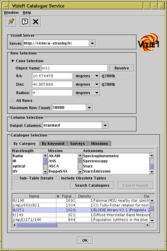
VizieR load dialogue
The VizieR query dialogue can be opened using the
VizieR Catalogue Service button ()
in the Load Window's toolbar
or the Control Window's VO menu.
It allows you to make queries directly to the
VizieR
service operated by
CDS.
VizieR is a comprehensive library of very many published astronomical
catalogues.
These items can equally be accessed from the web or other interfaces,
but this load dialogue makes it convenient to load data directly from
VizieR into TOPCAT.
Note that VizieR's idea of a catalogue is more complex than a single table; this means that in some cases querying one of VizieR's catalogues may result in more than one table being loaded into TOPCAT (the Sub-Table Details checkbox described below can help to control this).
The dialogue consists of four parts: the VizieR Server, Row Selection, Column Selection and Catalogue Selection panels, arranged top to bottom in the window. These are described below.
The VizieR Server panel allows you to specify which VizieR server you want to use for data download. By default the server at CDS is used, but there are mirrors elsewhere, whose URLs can be chosen from the selector. If you see a popup window complaining that the server cannot be contacted, you can choose a different one; you might also want to select one that is close to you for performance reasons.
The Row Selection panel specifies which rows you want to retrieve from the catalogue that you will select. You can choose one of the two radio buttons according to the kind of query that you want to make:
The Column Selection panel gives you some control over which columns will be included in the loaded table. This will include some or all of the columns the table has in the VizieR archive, and perhaps some standard ones added automatically by the service. The options are currently:
-out.add=_GLON,_GLAT would add galactic coordinates to the
standard set; see
https://vizier.cds.unistra.fr/doc/asu-summary.htx
for more details on VizieR hacking.
(In fact, this trick can be used to add VizieR parameters unrelated to
column selection as well).
The Catalogue Selection panel offers several different ways to identify which of the catalogues in the VizieR archive you want to query. In all cases you will be presented with a JTable of VizieR catalogues, and you must select one by clicking on the relevant row. You can sort within the displayed table by clicking on the column header. Note: for some of these options it is necessary to fill in the Row Selection panel before you can operate them (the controls will be disabled if no row selection has been made). That is because the catalogues listed will depend on the region you are going to query; VizieR is smart enough to know which catalogues have some coverage in the region in question. The options for catalogue selection are as follows:
Depending on the type of catalogue search you make, various attributes of the catalogues in question will be listed in the table for selection:
When you have made your selection of rows, columns and catalogue you can hit the OK button and TOPCAT will attempt to contact the VizieR service to load the resulting table or tables. You can cancel a request in progress with the Cancel button.
CDS make the following request:
If the access to catalogues with VizieR was helpful for your research work, the following acknowledgment would be appreciated: "This research has made use of the VizieR catalogue access tool, CDS, Strasbourg, France". The original description of the VizieR service was published in A&AS 143, 23 (2000).
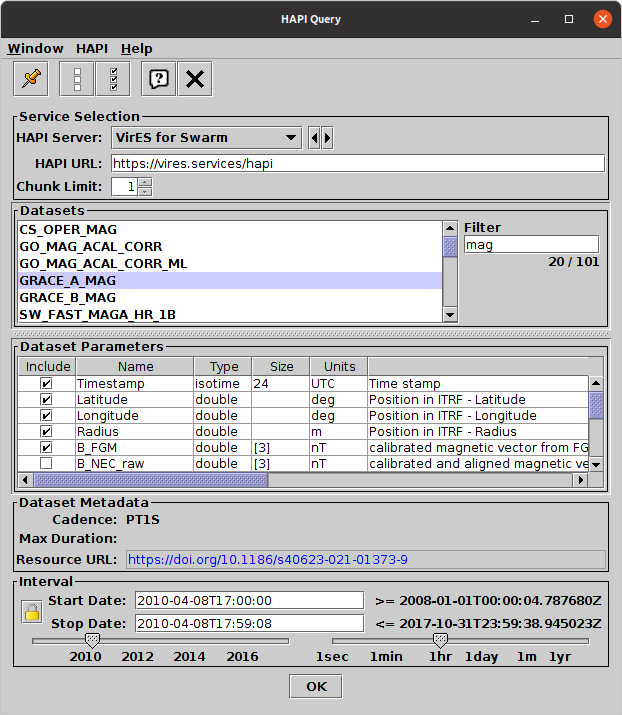
HAPI load dialogue
HAPI,
the Heliophysics Data Application Programmer’s Interface
is a protocol for serving streamed time series data.
This window is
opened using the HAPI Query button ()
in the Load Window's toolbar
or the Control Window's VO menu.
It lets you choose a HAPI service, select a dataset,
and request time series data over a given time range.
Queries can optionally be broken up into chunks to allow
download of datasets larger than that allowed in a single download
by the service.
The window is divided into the following parts.
To the right of the listing, search text may be entered into the Filter field to restrict the datasets listed (it is not case-sensitive). The text below gives the visible and total number of datasets available from the service.
There is also a column of checkboxes marked Include.
This determines which parameters will be included when the data is
downloaded; if you don't need them all, you can uncheck some of the
items (the initial timestamp item is always included).
As a convenience, the toolbar buttons
Select All () and
Unselect All () will check/uncheck
all of the items at once.
yyyy-mm-ddThh:mm:ss or yyyy-dddThh:mm:ss
in which any of the trailing parts can be omitted,
so for instance "2001-01-01" or "2001-01-01T16"
are both allowed.
The minimum and maximum values allowed for the selected dataset
are displayed to the right of the Start/Stop fields;
the entered values must fall within these bounds.
As an alternative to typing in the dates, you can use the sliders at the bottom: the left hand one selects the start date, and the right hand one selects the length of interval. Or you can use the sliders to set an approximate interval and then edit the dates by hand.
The Lock button () prevents the
Start/Stop dates fields from being updated automatically by the sliders
or as a consequence of changing datasets,
and can be useful when you are entering dates by hand.
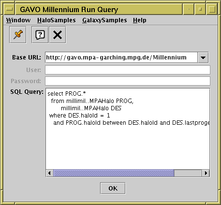
Virgo-Millennium load dialogue with an example query on the milli-Millennium database
This dialogue, selected from the
Load Window's toolbar
button () or the main VO menu,
permits direct SQL queries to a family of services
hosting cosmological simulation databases.
These services were originally developed by
GAVO,
the German Astrophysical Virtual Observatory,
and hold results from the Millennium, Virgo and EAGLE simulations.
Options are currently available to query services from
MPA Garching
and
Durham.
To make a query, fill in the fields as required:
http://gavo.mpa-garching.mpg.de/Millennium)
http://gavo.mpa-garching.mpg.de/MyMillennium)
http://virgodb.dur.ac.uk:8080/MyMillennium)
http://virgodb.dur.ac.uk:8080/Eagle)
The HaloSamples and GalaxySamples menus provide some examples of queries on the Milli-Millennium database (these have been copied from the GAVO query page). If you select one of these the SQL Query panel will be filled in accordingly.
Much more documentation, including tutorials, descriptions of the database schemas, and information about registering for use of the authenticated services, is available online. The MPA-Garching services are documented at http://gavo.mpa-garching.mpg.de/Millennium/Help, and the Durham services at http://virgodb.dur.ac.uk/.
Provided with TOPCAT are some example tables,
which you can access in a number of ways.
The simplest thing is to start up TOPCAT with the
"-demo" flag on the command line, which will cause
the program to start up with a few demonstration tables already loaded in.
You can also load examples in from the Examples menu in the Load Window however. This contains the following options:
Note these examples are a bit of a mixed bag, and are not all that exemplary in nature. They are just present to allow you to play around with some of TOPCAT's features if you don't have any real data to hand.
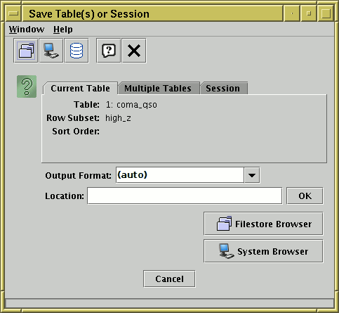
Save Window
The Save Window is used to write tables out,
and it is accessed using the Save Table button ()
in the Control Window's toolbar or
File menu.
The window consists of two parts. At the top is the Content Panel, which is used to determine exactly what table or tables are going to be saved, and below it is the Destination Panel, which is used to determine where they will be saved to. These panels are described separately in the subsections below.
For large tables, a progress bar will be displayed indicating how near the save is to completion. It is not advisable to edit tables which are being saved during a save operation.
In some cases, saving the table to a file with the same name as it was loaded from can cause problems (e.g. an application crash which loses the data unrecoverably). In other cases, it's perfectly OK. The main case in which it's problematic is when editing an uncompressed FITS binary table on disk. TOPCAT will attempt to warn you if it thinks you are doing something which could lead to trouble; ignore this at your own risk.
If you save a table to a format other than the one from which it was loaded, or if some new kinds of metadata have been added, it may not be possible to express all the data and metadata from the table in the new format. Some message to this effect may be output in such cases.
There is no option to compress files on output. You can of course compress them yourself once they have been written, but note that this is not usually a good idea for FITS files, since it makes them much slower to read (for TOPCAT at least).
The Content Panel is the upper part of the save window, and it is used to select what table or tables you want to save. The options are described in the following subsections.
The Current Table save option
saves the table currently selected in the
Control Window.
What is written is the
Apparent Table corresponding to the current table,
which takes into account any modifications you have made to
its data or appearance this session.
The current Row Subset and Sort Order
are displayed in this window as a reminder of what you're about to save.
Information about Row Subsets themselves and hidden columns will not
be saved, though you can save information about subset membership
by creating new boolean columns based on subsets
using the To Column button () from the
Subsets Window.
Alternatively you could use the Session Save
option described below.
The Multiple Tables save option allows you to save multiple tables to the same file. If a FITS or VOTable based output format is used, this means that when the file is loaded back into TOPCAT, all the saved tables will be individually loaded in.
The list of loaded tables is shown, with a column of checkboxes on the left. By default these are selected, but you can select or unselect them by clicking. The Select All and Unselect All buttons are also provided for convenience. When the save is performed, only those tables with the checkbox selected will be saved.
As with the Current Table save, it is the Apparent Table in each case which is saved, so that only unhidden columns, and rows in the Current Subset will be included. On the right hand side of the table is information to remind you which row subset and ordering will be saved.
The Session save option allows you to save much of the information about the loaded tables in your current TOPCAT session. Unlike the Current Table or Multiple Tables options, the whole of each loaded table, along with other information about your use of it, is saved, rather than just the Apparent Table. The saved items include:
The list of loaded tables is shown, with a column of checkboxes on the left. By default these are selected, but you can select or unselect them by clicking. The Select All and Unselect All buttons are also provided for convenience. When the save is performed, only those tables with the checkbox selected will be saved.
The tables are saved as a multi-table fits-plus (recommended) or VOTable file. This is a normal multi-table file in that any FITS or VOTable reader can read the tables it contains, but it contains some specialised metadata encoding information of special significance to TOPCAT, marking it as a saved session. The upshot is that if you save a file in this way and then load it back into TOPCAT, the tables it loads will appear in very much the same state as when you saved them, in terms of defined and current subsets, row order, visible and invisible columns, and so on. If you process it with some application other than TOPCAT, it will look quite like the table you saved, but with some additional data and metadata.
Note however that the reloaded state is not identical to that before saving. Only state belonging to tables is saved, so that for instance the state of Plot and Match windows will not be restored, and table activation actions are not saved either. It is possible that some of this may be changed in future releases.
The session save format has changed at TOPCAT version 4.5. Up to v4.4, columns and row subsets that had been defined algebraically were saved as fixed values, so the expressions were lost and it was no longer possible to edit them following a session save/load. At v4.5, the expressions themselves are saved and reloaded, which means the state is preserved better after a session save/load cycle, and may also result in smaller saved files. Post-v4.5 versions of TOPCAT should be able to load sessions saved by pre-v4.5 versions, but not vice versa. This also means that if you try to load a v4.5-format session into a non-TOPCAT reader, the algebraically-defined columns will not appear, but session-saving is not recommended for use with other table applications in any case.
The Destination Panel is the lower part of the save window, and is used to select where and how the table or tables should be saved.
The Output Format selector is used to choose the format in which the table will be written from one of the supported output formats. The available selections are somewhat different depending on what it is you are saving; for instance some formats cannot accommodate multiple tables, so these formats are not offered for the Multiple Table save. If the "(auto)" option is used, an attempt is made to guess the format based on the filename given; for instance if you specify the name "out.fits" a FITS binary table will be written. Usually just using (auto) or selecting one of the listed options will be appropriate, but you can type into the selector a more specific value with configuration options, for instance votable(format=BINARY,votable=V12); see the output format descriptions in Section 4.1.2 for more details.
You can specify the location of the output table in these ways, which are described in the following sections:
) to get a
browser
that shows you local and remote files) to get a
native browser
that uses your OS's standard file saving interface) to get the
SQL Output Dialogue
You can specify where to save a table by typing its location directly into the Output Location field of the Save Table window. This will usually be the name of a new file to write to, but could in principle be a URL or a SQL specifier.
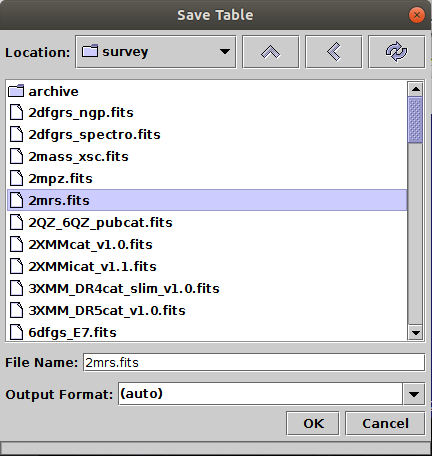
Filestore Browser for table saving
By clicking the Browse Filestore button in the Save Table window, you can obtain a browser which will display the files in a given directory.
The browser initially displays the current directory, but this can be
changed by typing a new directory into the File Name field,
or moving up the directory hierarchy using the selector box at the top,
or navigating the file system by clicking the up-directory button
or double-clicking on displayed directories.
The initial default directory can be changed by setting the
user.dir
system property.
The browser can display files in remote filestores such as on MySpace or SRB servers; see the section on the load filestore browser (Appendix A.6.1) for details.
To save to an existing file, select the file name and click the OK button at the bottom; this will overwrite that file. To save to a new file, type it into the File Name field; this will save the table under that name into the directory which is displayed. You can (re)set the format in which the file will be written using the Output Format selector box on the right (see Appendix A.7.2 for discussion of this selector).
By clicking the System Browser button or toolbar button
() in the
Save Window,
you can use your Operating System's native file browser to decide where
to save a file.
What this looks like is entirely dependent on your OS;
it may or may not contain system-specific features like shortcuts to
commonly-used directories.
Since TOPCAT has no control over the way this dialogue looks, it cannot contain the Output Format selector, and certain other things such as save cancel may not work as well as for the other dialogue types. To select the output table format, you will need to use the selector in the Save Window.
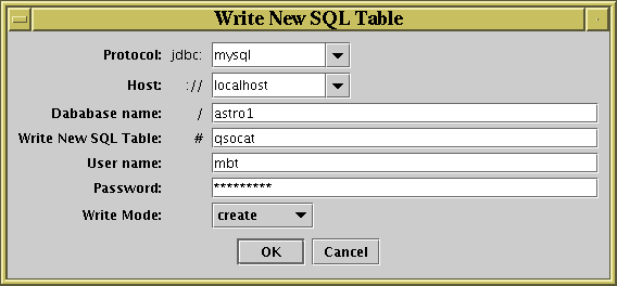
SQL table writing dialogue
If you want to write a table to an SQL database, you can use a specialised dialogue to specify the table destination by clicking the SQL Table button in the Save Table window.
This provides you with a list of fields to fill in which define the new table to write, as follows:
mysql" for MySQL's Connector/J driver
or "postgresql" for PostgreSQL's JDBC driver.
localhost" if the database is local).
There are a number of criteria which must be satisfied for SQL access to work within TOPCAT (installation of appropriate drivers and so on) - see the section on JDBC configuration. If you don't take these steps, this dialogue may be inaccessible.
This section documents the windows used to crossmatch rows either between two or more local tables or within a single table. This topic is discussed in more detail in Section 5. Windows for other kinds of joins are described elsewhere: concatenation in Appendix A.11.2 and matching with remote tables via VO services in Appendix A.9 and against VizieR and SIMBAD via the CDS X-Match service in Appendix A.11.1.
The next subsection describes the features which are common to the different types of match window, and the following subsections detail the operation of each distinct match window (internal, pair and multi-table).
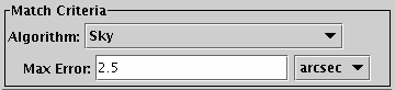
Match Criteria panel. The details will differ depending on what match type is chosen.
The match criteria box allows you to specify what counts as a match between two rows. It has two parts. First, you must select one of the options in the Algorithm selector. This effectively selects the coordinate space in which rows will be compared with each other. Depending on the chosen value, a number of fields will be displayed below, which you must fill in with values that determine how close two rows have to be in terms of a metric on that space to count as a match.
The following match types (algorithm values) are offered:
Note that in TOPCAT versions 4.3-5 and earlier a linear unscaled distance combination was used here, which did not give very meaningful Best match results.
Note that in TOPCAT versions 4.3-5 and earlier a linear unscaled distance combination was used here, which did not give very meaningful Best match results.
Depending on the match type, the units of the error value(s) you enter may be significant. In this case, there will be a unit selector displayed alongside the entry box. You must choose units which are correct for the number you enter.
More information is available in the GUI as a tooltip by hovering with the mouse pointer over the field in question.
See Appendix A.8.1.3 for information on optional tuning parameters which are sometimes displayed in this panel.
The matching framework is capable of performing even more complicated types of match, for instance Sky + 6-dimensional anisotropic Cartesian. These are not offered purely to avoid complicating the GUI. More flexible matching requirements in this in and other respects can be achieved by using the matching commands in STILTS instead.
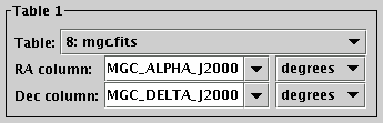
Column Selection Box. The details will differ depending on what match type is chosen.
The column selection boxes allow you to select which of the columns in the input tables will provide the data (the coordinates which have to match). For each table you must select the names of the required columns; the ones you need to select will depend on the match criteria you have chosen.
For some columns, such as Right Ascension and Declination in sky matches, units are important for the columns you select. In this case, there will be a selector box for the units alongside the selector box for the column itself. You must ensure that the correct units have been selected, or the results of the match will be rubbish.
In some cases these column and/or unit selectors may have a value filled in automatically (if the program thinks it can guess appropriate ones) but you should ensure that it has guessed correctly in this case. Only suitable columns are available for choosing from these column selectors; in most cases this means numeric ones.
Instead of selecting a column name from the list provided in these boxes, you may type in an expression. This can be a column name, or an algebraic expression based on column names, or even a constant. The expression language syntax is described in Section 7.
This subsection describes the use of some toolbar buttons available in the match windows:
 Tuning Parameters
 Full Profiling
 Parallel Execution
The parameters such as Max Error visible by default in the Match Criteria panel define what counts as a match and must be filled in for the match to proceed.
Optionally, you can see and adjust another set of parameters known as Tuning parameters. These will not affect the result of the match, but may affect its performance, in terms of how much CPU time and memory it takes. Most of the time, you can forget about this option, since TOPCAT attempts to pick reasonable defaults, but if your match is very slow (especially if it's unexpectedly slow given the sizes of the tables involved), or if it's failing with messages about running out of memory, then adjusting the tuning parameters may help.
To view the tuning parameters, use the
Tuning Parameters () toolbar button or
menu item. This will add display of tuning parameters to the
match parameters in the Match Criteria panel.
Suggested values are filled in by default, and may be affected by
the match parameters that you fill in; you can play around with
different values and see the effect on match performance.
If you do this, it is useful to use also the
Full Profiling () toolbar button to
turn on full profiling. This will cause additional information
on the amount of CPU time and memory used by each step to be
displayed in the logging panel at the bottom. There is a small
penalty in CPU time required to gather this information, which
is one reason it is not turned on by default.
What tuning parameters are available depends on the match type you have chosen. Some additional description is available as tooltips if you hover over the query field. In most cases, they are one or other of the following:
Even if you happen to have a good understanding of how the matching algorithm works (and you probably don't), this kind of tuning is a bit of a black art, and depends considerably on the details of the particular match. In some cases however it is quite possible to improve the time taken by a match, or the size of table which can be matched in a given amount of memory, by a factor of several. If you want to try to improve performance, try the default, adjust the tuning parameters slightly, look at how the performance changes by examining the logging output, and maybe repeat to taste.
Another thing which can affect speed and memory usage is whether your Java Virtual Machine is running in 32-bit or 64-bit mode. There are pros and cons of each - sometimes one will be better, sometimes the other. If you need to improve performance, experiment!
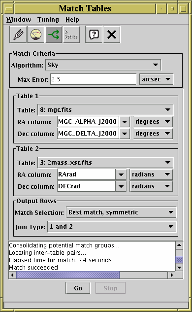
Pair Match Window
The Pair Match Window allows you to join two tables together
side-by-side, aligning rows by matching values in some of their
columns between the tables. It can be obtained using the
Pair Match () button in the
Control Window toolbar or
Joins menu.
In a typical scenario you might have two tables each representing a catalogue of astronomical objects, and you want a third table with one row for each object which has an entry in both of the original tables. An object is defined as being the same one in both tables if the co-ordinates in both rows are "similar", for instance if the difference between the positions indicated by RA and Dec columns differ by no more than a specified angle on the sky. Matching rows to produce the join requires you to specify the criteria for rows in both tables to refer to the same object and what to do when one is found - the options are discussed in more detail in Section 5.2.
The result is created from the Apparent versions of the tables being joined, so that any row subsets, hidden columns, or sorts currently in force will be reflected in the output. Progress information on the match, which may take a little while, is provided in the logging window and by a progress bar at the bottom of the window. When it is completed, you will be informed by a popup window which indicates that a new table has been created. This table will be added to the list in the Control Window and can be examined, manipulated and saved like any other. In some cases, some additional columns will be added to the output table which give you more information about how it has progressed (see Appendix A.8.2.1.
The Match Window provides a set of controls which allow you to choose how the match is done and what the results will look like. It consists of these main parts:
For information on the
Tuning Parameters (),
Full Profiling () and
Parallel Execution ()
toolbar buttons,
see Appendix A.8.1.3.
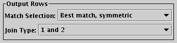
Pair match Output Rows Selector Box
When the match is complete a new table will be created which contains rows determined by the matches which have taken place. The Output Rows selector box allows you to choose on what basis the rows will be included in the output table as a function of the matches that were found.
In all cases each row will refer to only one matched (or possibly unmatched) "object", so that any non-blank columns in a given row come from only rows in the input tables which match according to the specified criteria. However, you have two choices to make about which rows are produced.
The Match Selection selector allows you to choose what happens when a row in one table can be matched by more than one row in the other table. There are four options:
The Join Type selector allows you to choose what output rows result from a match in the input tables.
Note that the choices of which Match Selection and Join Type to use are somewhat interlinked, and some combinations may not be very meaningful.
In most cases
(all the above except for 1 not 2 and 2 not 1),
the set of columns in the output table contains
all the columns from the first table followed by all the columns
from the second table. If this causes a clash of column names,
offending columns will be renamed with a trailing "_1" or
"_2".
Depending on the details of the match however,
some additional useful columns may be added:
Here is an example. If your input tables are these:
      X          Y         Vmag
      -          -         ----
   1134.822    599.247     13.8
    659.68    1046.874     17.2
    909.613    543.293      9.3
and
     X           Y         Bmag
     -           -         ----
   909.523     543.800     10.1
   1832.114    409.567     12.3
   1135.201    600.100     14.6
    702.622   1004.972     19.0
then a Cartesian match of the two sets of X and Y values with an error of 1.0
using the 1 and 2 option would give you a result like this:
     X_1       Y_1         Vmag    X_2        Y_2         Bmag    Separation
     ---       ---         ----    ---        ---         ----    ----------
   1134.822    599.247     13.8   1135.201    600.100     14.6     0.933
    909.613    543.293      9.3    909.523    543.800     10.1     0.515
using All from 1 would give you this:
     X_1       Y_1         Vmag    X_2        Y_2         Bmag    Separation
     ---       ---         ----    ---        ---         ----    ----------
   1134.822    599.247     13.8    1135.201   600.100     14.6     0.933
    659.68    1046.874     17.2
    909.613    543.293      9.3     909.523   543.800     10.1     0.515
and 1 not 2 would give you this:
     X         Y           Vmag
     -         -           ----
    659.68    1046.874     17.2
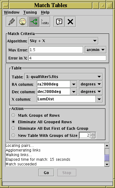
Internal Match Window
The Internal Match Window allows you to perform matching between
rows of the same table, grouping rows that have the same or similar
values in specified columns and producing a new table as a result.
It can be obtained by using the Internal Match
() item in the Control Window's
Joins menu.
You might want to use this functionality to remove all rows which refer to the same object from an object catalogue, or to ensure that only one entry exists for each object, or to identify groups of several "nearby" objects in some way.
The result is created from the Apparent versions of the tables being joined, so that any row subsets, hidden columns, or sorts currently in force will be reflected in the output. Progress information on the match, which may take some time, is provided in the logging window and by a progress bar at the bottom of the window. When it is completed, you will be informed by a popup window which indicates that a new table has been created. This table will be added to the list in the Control Window and can be examined, manipulated and saved like any other.
The window has the following parts:
When considering matching beyond pairs, see the comments in Section 5.4 about the semantics of multi-object matches.
For information on the
Tuning Parameters (),
Full Profiling () and
Parallel Execution ()
toolbar buttons,
see Appendix A.8.1.3.
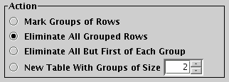
Internal Match Action Box
The Internal Match Action box gives a list of options for what will happen when an internal match calculation has completed. In each case a new table will be created as a result of the match. The options for what it will look like are these:
You can use this information in other ways, for instance if you
create a new Row Subset using the expression
"GroupSize == 5" you could select only those
rows which form part of 5-object clusters.
The Multiple Match Window allows you to perform matching between
more than two tables.
It can be obtained by using the Triple Match,
Quadruple Match etc () items
in the Control Window's
Joins menu.
The result is created from the Apparent versions of the tables being joined, so that any row subsets, hidden columns, or sorts currently in force will be reflected in the output. Progress information on the match, which may take some time, is provided in the logging window and by a progress bar at the bottom of the window. When it is completed, you will be informed by a popup window which indicates that a new table has been created. This table will be added to the list in the Control Window and can be examined, manipulated and saved like any other.
The window has the following parts:
See the comments in Section 5.4 about the semantics of multi-object matches.
For information on the
Tuning Parameters (),
Full Profiling () and
Parallel Execution ()
toolbar buttons,
see Appendix A.8.1.3.
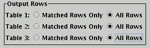
Multiple Match Action Box
The Multiple Match Action Box allows you to choose which rows appear in the output table following a successful multi-table match. For each input table you have two options to choose from:
At present the multi-table options available within TOPCAT are not
so comprehensive as those provided by the corresponding STILTS
command
tmatchn.
This may be improved in future.
Several windows in TOPCAT allow access to standard Virtual Observatory (VO) services. These share the idea of querying the Registry for suitable data services, selecting one of the services thus returned, and then submitting one or more queries to that data service to generate a tabular result. These ideas are explained in more detail in Section 6, while the current section describes the windows. The next subsection describes the components from which these windows are put together. All the windows contain a registry query panel to select a suitable data access service. The positional query windows also contain either a single or a multiple search panel, and the TAP window contains its own custom panel, to define the actual query or queries to submit to the selected service. The windows themselves are described in the following subsections.
TOPCAT also provides access to two important services provided by the CDS (Centre de Données astronomiques de Strasbourg): the VizieR Catalogue Service Query and CDS X-Match Upload Window. These are not strictly speaking Virtual Observatory services, but since they provide access to the comprehensive VizieR archive of astronomical tables they can provide similar or superior functionality to their VO counterparts, so it's worth being aware of them.
This section describes the graphical components which make up the VO data access windows.
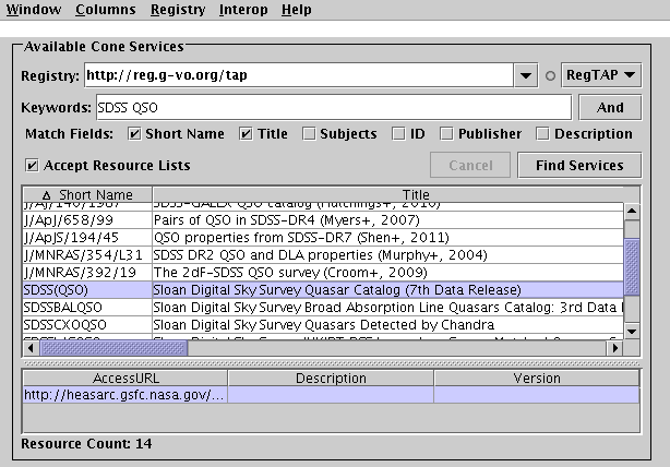
Registry Query Panel
The Registry Query Panel appears in all VO query windows (though by default the TAP window uses an alternative registry search panel) and allows you to search for entries in the Registry representing data services of the type appropriate to the window. Note that if you know the service URL for the service that you want to use, you don't need to use this panel at all; you can simply fill in the URL in the lower part of the window.
The top part of this panel contains the fields you can fill in to query the registry for services matching your constraints. This consists of the following parts:
To the right of this box is a selector that allows you to choose between two registry protocol options: RegTAP and RI1.0, corresponding to the IVOA Relational Registry and Registry Interface 1.0 standards respectively. At the time of writing (June 2014), RI1.0 is being phased out, and RegTAP is recommended. It is in any case considerably faster and more reliable than RI1.0. Unless you are a registry enthusiast, sticking to RegTAP is recommended.
The Update Registry List item in the Registry menu queries the currently selected registry for other registries, and adds more entries to the selector box as appropriate; the little round indicator between the URL and protocol selectors indicates progress of this query.
In some cases, when the window first appears, it will automatically query the registry for all known services of the appropriate type. This is currently the case for SIA and SSA services, since there is a manageable number of these. There are thousands of cone searches however, so for the cone search windows you need to fill in a query and submit it yourself. In either case, you can resubmit a query (hit the Cancel button first if necessary) to make another selection of registry entries.
When the query completes, a table of matching entries is displayed below the Submit button. The number of resources found is displayed at the bottom, labelled Resource Count. The table contains one row for each matching entry, i.e. each service of the appropriate type that you can submit your data query to. The columns in the table give a short name, title, description and some other information about each service. You can sort the table rows according to the entries in different columns by clicking on the column header; click again on the same header to reverse the sort order. A little up/down arrow in a column header indicates that that column is currently determining the sort order. You can adjust the columns which are visible using the Columns menu, or drag the columns sideways to change their order in the usual way.
You should select the service that you want to query for data by clicking on it. When this is done, you will see one or more rows appear in a second table underneath the first one. In most cases, this contains a single row which will be automatically selected. However, some registry entries have multiple data services associated with a single record - in this case you should select the appropriate entry from the lower table as well.
Once you have selected a data service in this way, its service URL will be entered in the lower part of the window (not shown in the figure above) and you are ready to perform the actual single or multiple data query.
If a SAMP hub is running (see Section 9),
it is possible to exchange lists of resources
between this window and other applications.
If another application sends a suitable message to TOPCAT, and the
resources are of an appropriate type, and the window is visible at the time,
the received list can be loaded and displayed here,
replacing any which are currently displayed.
You can control whether incoming lists are accepted and displayed in this
way using the Accept Resource Lists toggle,
either using the checkbox just above the resource display panel,
or using the corresponding item in the Interop menu.
If you wish to send your selection to one or more other applications
which can make use of them, use the
Broadcast Resource List () or Send Resource List ()
options in the Interop menu.
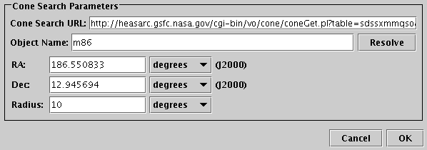
Single Positional Search Panel
The Single Positional Search Panel appears in VO-based table load dialogues and is used to specify data queries on a single region of the sky. The purpose is to load a new table (containing entries representing catalogue entries, images or spectra). To use it you must fill in the URL field and the position definition, and then hit the OK button.
&name=value parameters to it.
When the fields are filled in, hit the OK button and wait for the new table defined by your query parameters to load. If you get bored waiting (the service may be down, or just very slow, or you may have submitted a query with a very large return set), you can hit the Cancel button, and perhaps adjust the parameters and try again.
If a SAMP hub is running (see Section 9), then other running clients may be able to fill in the RA and Dec coordinates. For instance clicking on a sky position in an image viewing tool might fill in the sky position you clicked on. Usually this will happen automatically. This is often convenient, but may not be what you want. You can control whether incoming coordinate settings are accepted in this way using the Accept Sky Positions toggle below the Resolve button, or using the corresponding item in the Interop menu.
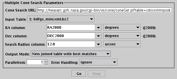
Multiple Positional Search Panel
The Multiple Positional Search Panel appears in VO-based multiple query windows which specify a procedure in which one query is made for each row of an input table. Each of the input rows defines a (probably small) region on the sky. The purpose is to find data records (about catalogue entries, images or spectra) in a remote catalogue corresponding to each row of a local catalogue. As such, it is used to define a kind of join, of a local Apparent Table with a remote one, where the remote one is exposed via a VO data service.
To use it you must fill in the URL field to select the remote service, and fields defining how each row of the input table can be turned into a positional query. You also need to define what form the result will be returned in. These parts are described below.
The URL field specifies the data service which is to be queried:
&name=value parameters to it.
The following fields define what queries are to be sent to the service:
The Output Mode selector indicates what will be done with the result.
The final controls adjust the details of how the individual queries are submitted to the remote service.
When all of the fields are filled in (defaults can be used for many of them), hit the Go button, and the search will commence. It may be quite slow; a progress bar is shown at the bottom of the window. When it completes, a popup window summarising the result will be shown. If you get bored waiting, you can hit the Cancel button, and perhaps adjust the parameters and try again.
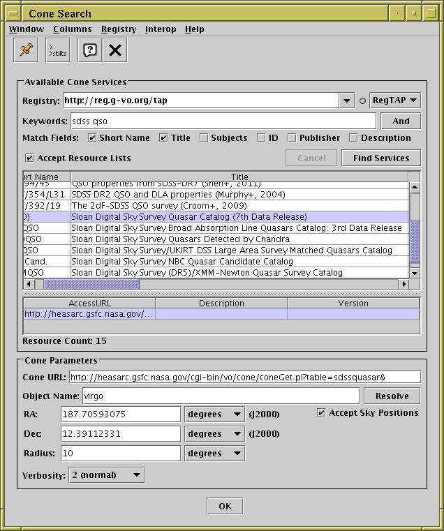
Cone table load dialogue
The cone search load dialogue can be opened using the
Cone Search button
() from the Load Window's toolbar or the Control Window's
VO menu.
It allows you to query one of a number of external web services for
objects from a given catalogue in a given region of the sky.
Data held by cone search services are effectively source catalogues
with sky position columns.
The window consists of a Registry Query Panel at the top, and a Single Positional Search Panel below.
The search panel includes a Verbosity selector as well as the normal features: this allows you to choose options for how many columns will appear in the output table, from 1 (minimum) to 3 (maximum). Some services will take notice of this parameter and return narrower or wider tables respectively, and others will ignore it.
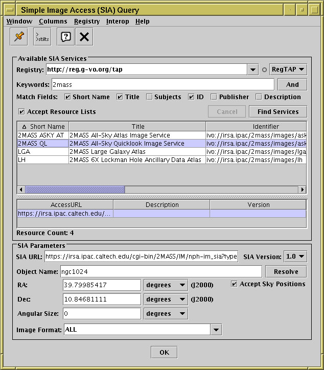
SIA query load dialog
The SIA query load dialogue can be opened using the
SIA Query button ()
from the Load Window's toolbar or the Control Window's
VO menu.
It allows you to query one of a number of external web services for
images covering a given region of the sky.
The window consists of a Registry Query Panel at the top, and a Single Positional Search Panel below. The Angular Size may be set to zero; this means that any image covering the chosen position will be selected. There is additionally an Image Format selector which allows you to restrict the result to contain only images in certain formats (the default is set to only FITS).
The result of a successful query is a table in which each row represents an image that can be downloaded from a remote site; one of the columns contains the image URL, and the other columns contain associated metadata such as image format, size, shape and so on. Different services provide different kinds of answer to these queries; some may have a static list of observed or reduced FITS files, and others may generate images on the fly. See the SIA standard, and individual registry records, for details. A useful thing to do with the resulting table might be to configure an activation action of Display Image or Send FITS Image.
TOPCAT supports two different (and incompatible) major versions of the SIA protocol, SIA version 1 and version 2. When you have selected a service to use, its protocol version number is displayed in the SIA Version indicator next to the SIA URL display. If you have entered the URL manually, you will need to make sure this is set to the appropriate value. Note that, although SIAv2 allows a number of query possibilities not offered by SIAv1, at present TOPCAT does not support this additional functionality for SIAv2 services.
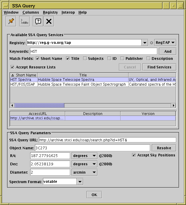
SSA query load dialog
The SSA query load dialogue can be opened using the
SSA Query button ()
from the Load Window's toolbar or the Control Window's
VO menu.
It allows you to query one of a number of external web services for
spectra in a given region of the sky.
The window consists of a Registry Query Panel at the top, and a Single Positional Search Panel below. The SSA specification says that the Diameter field may be left blank, in which case the service "should supply a default value intended to find nearby objects". However, experience shows that this doesn't always work, so it may be best to fill this in. It is also permitted to leave the RA and Dec fields blank, if you don't want to restrict the search by sky position. That may be a reasonable thing to do, for example, for services providing theoretical rather than observed spectra, or if you want all the data (subject to possible service restrictions). There is additionally a Spectrum Format selector which allows you to restrict the result to contain only spectra in certain formats. By default, the service chooses which formats to return.
The result of a successful query is a table in which each row represents a spectrum that can be downloaded from a remote site; one of the columns contains the spectrum download URL, and the other columns contain associated metadata such as spectrum format, WCS, provenance information and so on. See the SSA standard for details. A useful thing to do with the resulting table might be to configure an activation action of Send Spectrum.
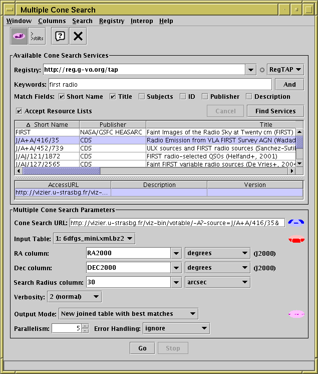
Multiple cone search window
The multiple cone search window can be opened using the
Multicone button ()
in the Control Window's toolbar, or its
VO or Joins menus.
It allows you to select one of a number of external web services which
provide remote catalogue queries, and execute a query for each row
of an input table.
This effectively allows you to perform a positional crossmatch between a
local table and a remote one.
The window consists of a Registry Query Panel at the top, and a Multiple Positional Search Panel below.
The search panel includes a Verbosity selector as well as the normal features: this allows you to choose options for how many columns will appear in the output table, from 1 (minimum) to 3 (maximum). Some services will take notice of this parameter and return narrower or wider tables respectively, and others will ignore it.
The following item is available in the toolbar and Search menu:
 Use Service Coverage
When in operation (i.e. when this option is selected and the service provides coverage information) the coverage of the service, input table and their overlap is summarised with small (Mollweide equatorial) all-sky icons in blue, red and magenta respectively, as in the screenshot above. This makes it easy to see the sky regions in which results may be obtained, and also the amount by which this option reduces useless queries.
Currently, this option effectively works only for cone searches provided by CDS's VizieR service (publisher "CDS") which provide coverage information using Multi-Order Coverage maps (MOCs). For non-VizieR services this option has no effect.
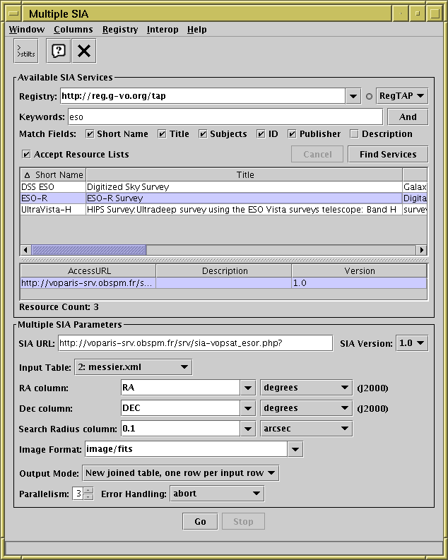
Multiple SIA window
The multiple Simple Image Access window can be opened using the
Multiple SIA button () from the Control Window's
VO or Joins menus.
It allows you to select one of a number of external web services which
provide queries on remotely accessible image holdings, and execute
a query for each row of an input table.
The window consists of a Registry Query Panel at the top, and a Multiple Positional Search Panel below. The Search Radius column may be set to zero; this means that any image covering the chosen position will be selected. There is additionally an Image Format selector which allows you to restrict the result to contain only images in certain formats (the default is set to only FITS).
The result of each single successful query is a table in which each row represents an image that can be downloaded from a remote site; one of the columns contains the image URL, and the other columns contain associated metadata such as image format, size, shape and so on. Different services provide different kinds of answer to these queries; some may have a static list of observed or reduced FITS files, and others may generate images on the fly. See the SIA standard, and individual registry records, for details.
Note that some services return multiple images at the same positions but at different wavelengths. In this case TOPCAT's criterion for the "best" match (the one closest to the central query position) may not make much sense. For this reason, take care if using the "New joined table with best matches" or "New joined table, one row per input row" output modes.
One use of this function is to add some columns to an existing table which contain URLs of images from a given server corresponding to the sky positions of those rows. Having done this you might want to configure an activation action for the resulting table of Display Image or Send FITS Image.
TOPCAT supports two different (and incompatible) major versions of the SIA protocol, SIA version 1 and version 2. When you have selected a service to use, its protocol version number is displayed in the SIA Version indicator next to the SIA URL display. If you have entered the URL manually, you will need to make sure this is set to the appropriate value. Note that, although SIAv2 allows a number of query possibilities not offered by SIAv1, at present TOPCAT does not support this additional functionality for SIAv2 services.
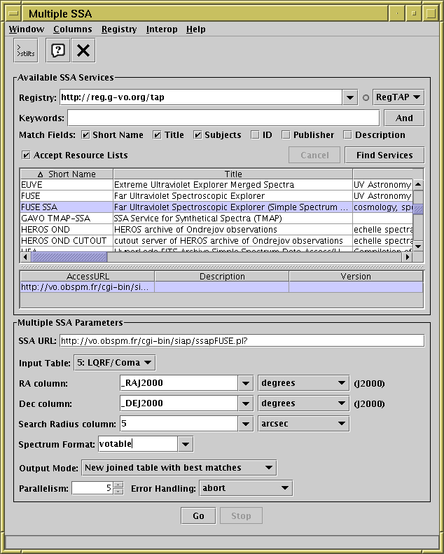
Multiple SSA window
The multiple Simple Spectral Access window can be opened using the
Multiple SSA button () from the Control Window's
VO or Joins menus.
It allows you to select one of a number of external web services which
provide queries on remotely accessible spectral data holdings, and execute
a query for each row of an input table.
The window consists of a Registry Query Panel at the top, and a Multiple Positional Search Panel below. The SSA specification says that the Search Radius column may be left blank, in which case the service "should supply a default value intended to find nearby objects". However, experience shows that this doesn't always work so it may be best to fill this in. There is additionally a Spectrum Format selector which allows you to restrict the result to contain only spectra in certain formats. By default, the service chooses which formats to return.
The result of each single successful query is a table in which each row represents a spectrum that can be downloaded from a remote site; one of the columns contains the specturm URL, and the other columns contain associated metadata such as spectrum format, WCS, provenance information and so on. See the SSA standard for details.
One use of this function is to add some columns to an existing table which contain URLs of spectra from a given server corresponding to the sky positions of those rows. Having done this you might want to configure an activation action for the resulting table of Send Spectrum.
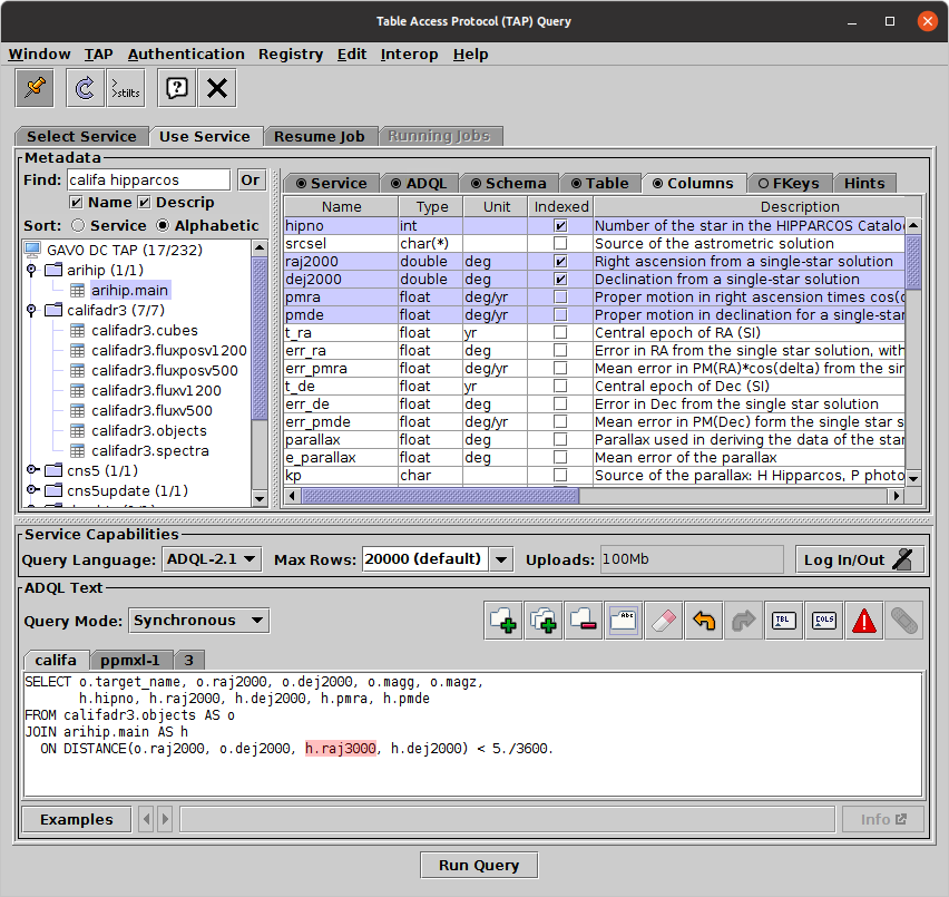
Table Access Protocol Window
The Table Access Protocol (TAP) load window can be opened using the
TAP Query button ()
in the Control Window's toolbar
or VO menu,
or the Load Window's toolbar.
It allows you to use the TAP protocol to
make freeform queries of remote database services
using an SQL-like language.
This is a powerful capability, giving you full access to
remote data holdings, and use of the
IVOA-endorsed TAP standard means that you can use
the same interface for many different remote datasets.
Using TAP is one of the more complicated things you can do in TOPCAT, but it's well worth getting to grips with because of the capabilities it gives you for customised access to all kinds of remote data.
In order to interrogate the remote database you will have to write queries in Astronomical Data Query Language (ADQL). ADQL is essentially a particular dialect of SQL, so if you have used SQL before, you should be able to write ADQL queries. A tutorial on writing ADQL/SQL is beyond the scope of this manual, but the Use Service tab provides a quick cheat sheet in the Hints tab of the metadata panel, and an Examples menu which will give you a good start in using it. There are introductions and tutorials elsewhere, for instance at http://docs.g-vo.org/adql (Markus Demleitner) and in the documentation of some TAP service web pages.
Once your query is written, you can submit it in either synchronous or asynchronous mode. Synchronous queries begin to execute right away and should have a relatively short runtime; asynchronous queries are submitted to a server, run for a potentially long time, and retrieve the result later.
The window is composed of four tabs, of which you can see one at a time (some of these tabs themselves contain tabbed parts). You will use two or three of them when submitting a TAP query. Each tab is described in more detail in the following subsections, but an overview of their operation is like this:
When you first visit this window, the Select Service tab will be visible, and when an asynchronous query has been submitted the Running Jobs tab will be visible. If you want to submit another query to the same service, or use a different service, just select Use Service or Select Service respectively, by clicking on the appropriate tab at the top.
This window offers some menus additional to the standard VO window menus:
)
detail-sensitive requests
to the /tables endpoint.
No detail specification is made initially,
so the service decides whether up-front loading is done.
Still compatible with VOSI 1.0 services.
detail-sensitive requests
to the /tables endpoint.
detail=max is specified initially to indicate that
full metadata up-front metadata load is preferred.
Still compatible with VOSI 1.0 services.
detail-sensitive requests
to the /tables endpoint.
detail=min is specified initially to indicate that
on-demand column load is preferred.
Still compatible with VOSI 1.0 services.
/tables endpoint of
the TAP service as defined by VOSI 1.0;
all table metadata is loaded up front.
/tables
as implemented (at time of writing) by the TAPVizieR service;
columns are read only when required
(experimental, may be withdrawn).
TAP_UPLOAD.* table) is performed.
The options
(TABLEDATA,
BINARY,
BINARY2)
correspond to the different defined VOTable serialization formats.
The choice shouldn't affect any results, but it may affect
required bandwidth and some services may (though shouldn't)
have non-standard requirements for serialization format.
Accept-Encoding: gzip
headers with most of the HTTP requests when communicating with the
TAP service. That ought to reduce required bandwidth considerably,
but only if the service chooses to honour this request.
The setting should have no effect on the actual results,
but may affect performance.
 )
)
)
)
Note: TAP is a complex protocol, and at time of writing, many TAP services still do not provide full and error-free implementations. Unexpected behaviour may be a result of service implementation deficiencies. Hopefully that will improve over time.
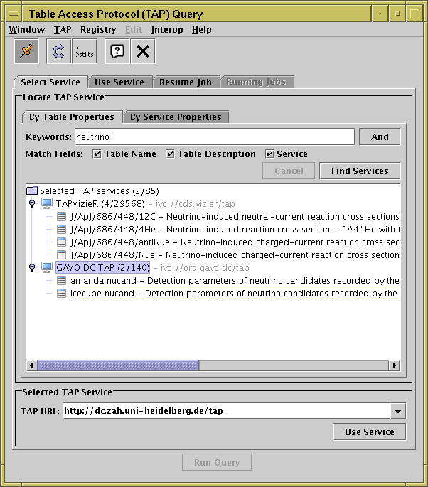
TAP window with Select Service tab visible
The Select Service tab of the TAP load dialogue allows you to choose which TAP service you wish to query. You need to do this before submitting a new TAP query.
There are two separate tabs within the Locate TAP Service sub-panel, corresponding to two different ways to select the service you want to use.
If you know the URL of the TAP service you wish to query, you can enter it directly into the TAP URL field at the bottom of the window without a registry search. This field remembers URLs previously entered into it, so if you click the little down-arrow on the right, you can easily return to services you visited earlier in the same session. The state (entered ADQL etc) of those sessions is also retained.
Once a service URL has been chosen in one of these ways, you can click the Use Service button at the bottom (or equivalently the tab header at the top), and you will be moved to the Use Service tab.
TAP window with Use Service tab visible
The Use Service tab of the TAP load dialogue displays information about the service you have selected to query, including what tables are available and what columns they contain, and allows you to enter the query text and some additional options about how the query is to be executed. Once you have entered suitable query text, click the Run Query button at the bottom of the window to submit the job.
The various parts of the window are described in detail below.
The Metadata panel displays information about the tables held by the selected service. On the left of the panel is a searchable tree summarising the schemas and tables in the service, and on the right are some tabs containing more detail. Note all this information has to be loaded from the server, so in some cases you may have to wait before it is visible.
The tree on the left contains a listing of the service's Schemas, and under them the Tables they contain. A Schema in this context is just a subject grouping that contains one or more tables. Each schema notes in brackets the number of tables it contains; you can reveal or hide the tables by clicking on the schema node's handle. If the service contains only a small number of tables it may be convenient just to scroll up and down to see them all. But for services with hundreds or thousands of tables, you might need some help to find the tables that you're interested in by using the controls above the tree:
To the right of the tree is a tabbed panel giving detail relating to the currently selected tree node. Select a tree node by clicking on it. Each tab has a little circle next to the title which may be empty or filled, according to whether it contains information. If it's empty it's either because that information doesn't make sense for the selected node in the tree (e.g. if a schema is selected, there is no column information) or because the information has not been retrieved from the service; either it's on its way and will be filled in later, or there's an error. The tabs are as follows:
 )
in the panel will try to open the relevant pages in
an external web browser (or you can copy and paste them yourself).
The content of this tab is not sensitive to which node of the tree
is currently selected.
).
The content of this tab is not sensitive to which node of the tree
is currently selected, but it may change according to which
ADQL version is selected.
)
in the panel will try to open the relevant pages in
an external web browser (or you can copy and paste them yourself).
The content of this tab is not sensitive to which node of the tree
is currently selected.
).
The content of this tab is not sensitive to which node of the tree
is currently selected, but it may change according to which
ADQL version is selected.
mag
click on the Unit column header.
If no table is selected in the tree, this tab will be empty.
The Service Capabilities panel shows capability metadata that the service provides about itself. This has to be loaded from the server and may not appear immediately. It contains the following information:
TOP nnn" is used in the ADQL,
the nnn limit may override the value supplied here.
The ADQL Text panel is where you can enter the actual query text for the request. It has the following parts:
SELECT COUNT(*) FROM table);
the result of the query is the row count in a one-column, one-row table,
and there's not much point loading that table into TOPCAT.
 Add Tab
 Copy Tab
 Remove Tab
 Title Tab
 Undo
Undo
 Redo
Redo
 Insert Table
 Insert Columns
 Parse Errors
 Fix Errors
As you enter the query text, it will be checked for syntax errors.
If an error is found, the place in the text which appears
to have caused it
will be highlighted in pink (as in the figure above).
To see more detail on the error,
click the Parse Errors () button.
In some cases, the parser can guess how to fix such errors;
if the Fix Errors () button is enabled,
you can try clicking that.
The checking itself is reasonably reliable, but the position of the highlighted error, and the text of the error message, can sometimes be a bit misleading, so don't take the details too seriously. The error highlighting is just used as a warning, you are not prevented from submitting a query marked as erroneous, since in some cases TAP services may accept ADQL which is not strictly correct, and in some cases the error checking may not be perfect. Note also that for various reasons the service may not be able to accept all queries that count as syntactically valid ADQL, so even if TOPCAT doesn't report any errors, the service may still respond with an error message.
The details of the syntax checking depend on the table metadata, ADQL version and optional language features declared by the service. If multiple ADQL versions are available in the Query Language selector, it is also be possible to change the language version checked by making a different selection.
The Examples menu is divided into a number of sub-menus, though not all will be enabled for all services. The sub-menus are:
ivoa.obscore table),
which describes astronomical observations in a standardised way.
You can use these to do things like search for all observations
at a particular sky position, or observation time, or waveband etc.
Only available if the service declares support for the ObsCore
data model.
rr schema).
You can use these to do things like search for
all TAP services containing tables having columns with particular
physical meanings,
or all cone search services relating to particular wavebands, etc.
You can use queries like this to perform more sophisticated searches
for TAP services than you can do using the
Select Service tab.
Only available if the TAP service declares support for the RegTAP
data model (i.e. if it hosts an IVOA searchable registry).
When you select an example from one of the sub-menus, its name and title will be displayed to the right of the Examples button. Little left and right arrow buttons allow you to cycle through the examples in the current submenu so you can browse what's available.
Some examples come with additional explanation on the web.
If the example you're currently looking at has such additional
documentation then the Info button
to the right will be enabled, and clicking on that should open
the relevant page in a browser on your desktop.
Some TAP services permit Table Uploads.
What this means is that you can upload tables from TOPCAT into the
remote database and perform queries on your table directly.
In this way you can perform joins between your own tables
(anything loaded into TOPCAT) and any of the tables in the remote
database. This is an extremely powerful feature.
To take advantage of it, you just need to use a special form for
the table name to reference a TOPCAT-based table:
you write "TAP_UPLOAD.t<n>", where
<n> is the ID number of the table in TOPCAT,
that is the number before the colon in the
Control Window Table List.
If the table's label has a suitable form
(roughly, if it's alphanumeric and unique)
you can use that instead of "t<n>".
So, if a table is identified as "1: messier"
in the table list, you can reference it in ADQL as
"TAP_UPLOAD.t1" or as "TAP_UPLOAD.messier"
- see the Upload
sub-menu of the Examples menu described above for
some examples.
Note the table uploaded in this way is the
Apparent Table corresponding to the
given ID number, i.e. current subset and column selections apply.
It's a good idea to ensure that any table you are uploading has
columns with sensible names, otherwise the service may rename the
columns or otherwise have trouble handling it.
Some TAP services (at time of writing, a minority) permit or require you to log in before using the service, as discussed in Section 6.3. The behaviour of this window depends on whether the service provides mandatory, optional or no authentication, and can be controlled using the Log In/Out button on the right of the Service Capabilities panel in the middle of the window.
)
to supply your username and password.
The advantage that authenticating confers on your usage
depends on the service;
in some cases you will have access to more of the hosted data,
in other cases it may entitle you to higher resource limits or
enable protection of your asynchronous query results.
TOPCAT can't tell you what the difference will be if you authenticate,
but following successful login it will reload and display
the service metadata in case it has changed for the
new authenticated context.
The Log In/Out button's appearance changes depending
on whether you are logged in ( ) or not ().
To check your authenticated identity, you can hover over the button
or look under the Authentication item in the
Service tab of the Metadata Panel above.
) or not ().
To check your authenticated identity, you can hover over the button
or look under the Authentication item in the
Service tab of the Metadata Panel above.
If you have already logged in, clicking this button will pop up the authentication dialogue again and you can enter a different username and password, or select Anonymous to log out. It is also possible to log out of all services you are currently authenticated with by using the Reset Authentication option from the Authentication menu.
Note: These authentication arrangements in TOPCAT are new at version 4.9, and rely on VO standards that are still under discussion. The behaviour and user interface may change in future releases, and at time of writing not all TAP services that provide authentication advertise it in a way that TOPCAT can work with. It is hoped that authentication interoperability will improve in future versions of TOPCAT and of server-side software.
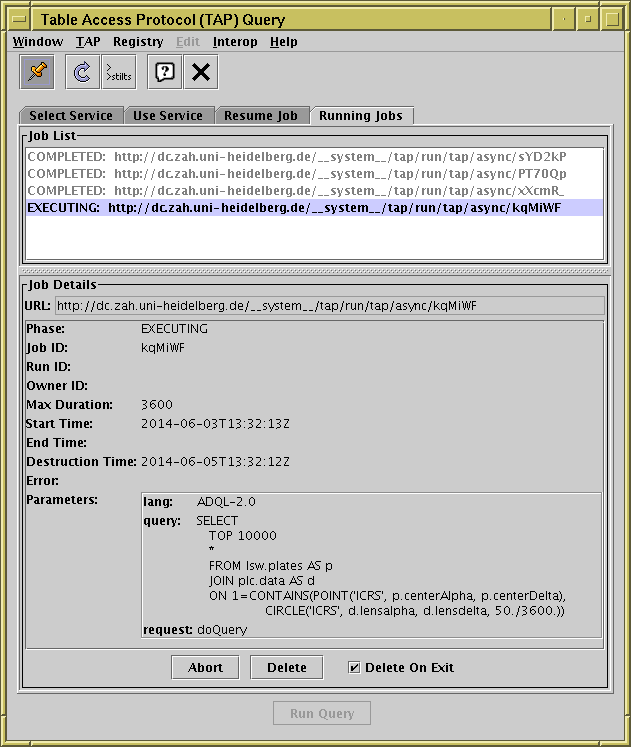
TAP window with Running Jobs tab visible
The Running Jobs tab of the TAP load dialogue shows a list of the asynchronous jobs you have submitted, with information about their current progress.
The upper part of the screen shows a list of the jobs submitted, along with a one-word summary of their status (their Phase). If one of these jobs is selected, its details will be shown in the lower part. By default the most recently submitted job will be shown, but you can select a job by clicking on it.
The information displayed is retrieved from the server, and can only be seen as long as the job has not been deleted, either by you the user, or as a result of server policy (for instance a maximum job lifetime). The following items, if provided by the service, are shown:
There are three buttons at the bottom of the screen which affect the status of the currently displayed job:
If no jobs are currently visible (none have been submitted or they have all been deleted), this tab is inaccessible.
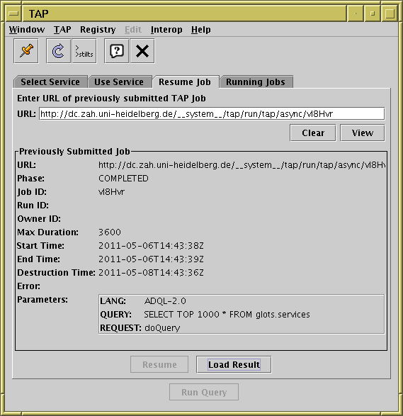
TAP window with Resume Job tab visible
The Resume Job tab of the TAP load dialogue allows you to continue execution of an asynchronous job which was started outside of this run of TOPCAT, either during an earlier TOPCAT run, or using some other mechanism. This may be useful if you have submitted a long-running job on an earlier day or on a different machine and want to monitor its progress or pick up the results.
To use it, enter the Job URL into the URL field at the top and click the View button. If a job with that URL exists, its details will be displayed in the panel below, in the same format as for the Running Jobs tab.
Depending on whether the job has completed or not, either the Resume or Load Result button at the bottom of the window will be enabled. You can click the appropriate one either to monitor its progress further or to pick up the completed result.
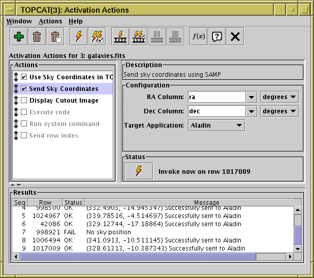
Activation Window
The Activation Window lets you configure what happens when a
row is activated.
You can display it using the
Activation Window ()
button when the chosen table is selected in the
Control Window's Table List.
A list of suggested Activation Actions is displayed in the top left panel, and if you select one of these its details, including configuration and invocation options and the results of invoking these actions to date, will be shown in the rest of the window. Those actions in the list which are enabled (not greyed-out) and have their checkbox checked will be invoked every time a table row is activated. Unchecked ones can be invoked manually. More description of each of the panels is given below.
The Actions list
lists a number of activation actions that may be appropriate
for the table this window applies to.
Others, including duplicates of ones already listed,
can be added from the Add Action () button
or menu item.
The only reason the full list is not visible by default is to
avoid too much clutter in the window.
Each action has a checkbox; if checked, an attempt will be made to
invoke that action whenever a row is activated (e.g. clicked on).
If the checkbox is not checked, the action can still be invoked
manually for the current row using the
Invoke Selected Action on Current Row ( ) or
Invoke Selected Action on All Rows (
) or
Invoke Selected Action on All Rows ( ) buttons.
If the action name is greyed out, it means that it can't currently
be invoked for some reason, perhaps because it needs more configuration first.
To find out the reason, look in the Status panel,
which should have a helpful message indicating why it's disabled.
The grab handles () can be used to re-order items in the
list, though this order doesn't have much effect except visually.
Actions can be removed from the list by selecting them and using the
Remove Current Action () button.
) buttons.
If the action name is greyed out, it means that it can't currently
be invoked for some reason, perhaps because it needs more configuration first.
To find out the reason, look in the Status panel,
which should have a helpful message indicating why it's disabled.
The grab handles () can be used to re-order items in the
list, though this order doesn't have much effect except visually.
Actions can be removed from the list by selecting them and using the
Remove Current Action () button.
The Description panel gives a short description of the behaviour of the currently selected action.
The Configuration panel displays a user interface to configure the details of what the selected action will do. The format depends on the action; see Appendix A.10.1 for details.
The Status panel contains a button (identical to that in the toolbar) that will invoke the currently selected action on the most recently activated row (or the first row, if no row has been activated so far in this table). It may be in one of two states. If the action is sufficiently configured to be used immediately, the button will be enabled, and clicking on it will cause the action to happen immediately, with the result being displayed in the Results panel below. However, if the action cannot be performed for some reason, the button will be greyed out, and some text will explain why it's disabled. Sometimes that means that the configuration in the panel above needs to be adjusted (e.g. some values filled in).
The Results panel
contains a line added every time the currently selected action is invoked,
either by the Invoke buttons
(,  ,
,
,
,  )
or because a row has been activated elsewhere in the application.
Each line contains four entries:
)
or because a row has been activated elsewhere in the application.
Each line contains four entries:
A Security panel may occasionally also be visible. If you see this, consult Appendix A.10.3 for an explanation.
The following items are available in the toolbar or menus:
Add Action
Remove Selected Action
 Remove Inactive Actions
 Approve All Actions
Invoke Selected Action on Current Row
Activate Current Row
Invoke Selected Action on All Rows
Activate All Rows
Approve All Actions
Invoke Selected Action on Current Row
Activate Current Row
Invoke Selected Action on All Rows
Activate All Rows
 Pause Sequence
 Cancel Sequence
Available Functions
Cancel Sequence
Available Functions
All the state of this window is saved and restored if you save its corresponding table using the Save Session option.
A range of activation actions is available.
Which ones are displayed for selection by default depends on the
characteristics of the table, but if you want to use one that's not
displayed, you can use the Actions|Add Action ()
menu item to insert it into the list.
The available actions are listed in the following sections.
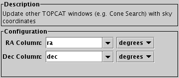
Configuration for Use Sky Coordinates in TOPCAT action
The Use Sky Coordinates in TOPCAT action causes the sky coordinates of an activated row to be communicated to certain other TOPCAT windows that have sky position entry widgets, for instance to update the query position in the Cone Search and Simple Image Access windows, and to be used as the default position in certain queries from the Examples menu in the TAP window.
This is in most cases useful behaviour so if sky coordinates can be identified this action will be enabled by default. If you find it unhelpful however (e.g. you have typed a position into the Cone Search window position selector and you don't want it to be overwritten) it can be disabled.
Configuration:
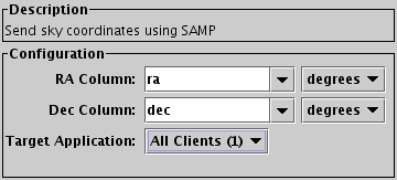
Configuration for Send Sky Coordinates action
The Send Sky Coordinates action causes the
sky coordinates associated with the activated row to be
sent using SAMP to one or all suitable applications.
It sends a message with the MType coord.pointAt.sky,
so at least one external SAMP client subscribed to such messages
must be registered.
One way to use this action is to configure it to transmit to a viewer of all-sky imagery such as Aladin. Then whenever a row is activated, Aladin will change its view to show imagery at the sky coordinates corresponding to that row.
Configuration:
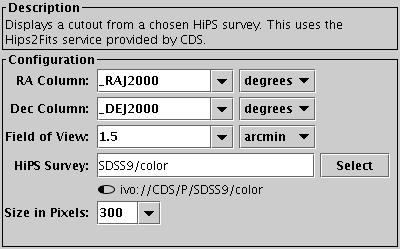
Configuration for Display HiPS Cutout action
The Display HiPS Cutout action uses the hips2fits service at CDS to acquire a resampled image at the activated row's sky (or planetary) position and displays it in a no-frills image viewer window. The data is taken from a Hierarchical Progressive Survey (HiPS), an all-sky image data set. There are several hundred HiPS available providing imagery for many important sky and planetary survey datasets, so this easy to use activation action is often a good option for viewing imagery associated with activated positions.
Configuration:
Alternatives:
The hips2fits service is very flexible.
If this action doesn't invoke it in exactly the way
you want it to, you can customise the behaviour by using the
Display Image action instead
constructing your own custom hips2fits URL,
perhaps by using the hips2fitsUrl function from the
URLs class.
You can also use the
Send HiPS Cutout action
if you want to view the image in an external viewer such as Aladin or ds9.
If you want to be able to zoom around the HiPS image however,
the best thing might be to open the HiPS in
Aladin and use the
Send Sky Coordinates action
to communicate with it.
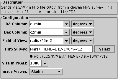
Configuration for Send HiPS Cutout action
The Send HiPS Cutout action uses the hips2fits service at CDS to get the URL of a resampled image at the activated row's sky position and asks an external image viewer application to load it via SAMP. The data is taken from a Hierarchical Progressive Survey (HiPS), an all-sky image data set.
Since the Aladin viewer already has all-sky viewing of HiPS datasets built in, you may find it better to load the HiPS directly into Aladin and use the Send Sky Coordinates action to communicate with it.
Configuration:
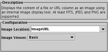
Configuration for Display Image action
The Display Image action uses the contents of a column to provide a URL or filename giving the location of an image to display in an internal viewer. The image can be in a graphics format such as JPEG, PNG, or GIF, or it can be a FITS image. The standard image support is implemented by Java's ImageIO library, so the details of installation determine what formats are supported. Java version 9 has more extensive image format support than earlier Java versions.
Note that for more sophisticated image handling, especially for FITS images, the Send FITS Image option in conjunction with an external image viewer application may be more appropriate.
Configuration:
< convert " + filename + " -normalize png:-",
using the ImageMagick convert command.
This rather advanced usage may only work on Un*x-like OSs.
This option is usually not required, and has security implications;
if it is used in an action loaded from a session file,
the security panel
will be displayed.
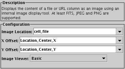
Configuration for Display Image Region action
The Display Image Region action behaves like Display Image, but additionally identifies an X/Y position on the displayed image, in pixel coordinates. This is currently done by scrolling the image if necessary to ensure the identified position is in view, and highlighting it with green crosshairs.
Configuration:
< convert " + filename + " -normalize png:-",
using the ImageMagick convert command.
This rather advanced usage may only work on Un*x-like OSs.
This option is usually not required, and has security implications;
if it is used in an action loaded from a session file,
the security panel
will be displayed.
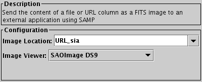
Configuration for Send FITS Image action
The Send FITS Image action takes a URL or filename
in the table that points to a FITS image,
and sends it using SAMP
to an external image viewer for display.
It sends a message with the MType image.load.fits,
so at least one external SAMP client subscribed to such messages
must be registered.
Suitable image viewers for use with this action include Aladin, GAIA and SAOImage DS9.
Configuration:
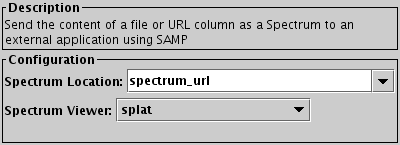
Configuration for Send Spectrum action
The Send Spectrum action takes a URL or filename
in the table that points to a spectrum resource,
and sends it using SAMP
to an external viewer for display.
The supported spectrum data formats are dependent on the
external application in question.
It sends a message with the MType spectrum.load.ssa-generic,
so at least one external SAMP client subscribed to such messages
must be registered.
Suitable spectrum viewers for use with this action include SPLAT and VOSpec.
Configuration:
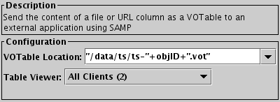
Configuration for Send VOTable action
The Send VOTable action takes a URL or filename
in the table that points to a VOTable document,
and sends it as a table using SAMP
to an external program to load.
It sends a message with the MType table.load.votable,
so at least one external SAMP client subscribed to such messages
must be registered.
This action can be used to send tables to other running instances of TOPCAT, or to different applications such as Aladin, GAIA or SAMP-enabled Python scripts.
Configuration:
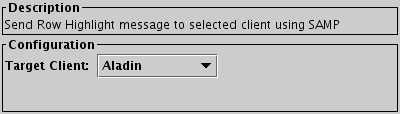
Configuration for Send Row Index action
The Send Row Index action sends a message to
other SAMP applications giving the row
index of the activated row.
This is in general only useful to other applications if they are
already aware of the table whose row indices are being communicated
like this, so a usual pattern of usage would be first to
send the table to one or several external applications,
and then to set up this action to indicate which rows are being
selected. If it is known that the table in question has never
been communicated to other applications, the action will be disabled.
The message sent has the MType table.highlight.row,
so at least one external SAMP client subscribed to such messages
must be registered.
Suitable clients for use with this action include image viewers
such as
Aladin,
GAIA
and
SAOImage DS9.
If you send a table to one of
(e.g. using the Broadcast Table ()
button in the Control Window toolbar)
and then set up this action to send row indices,
then the image viewer will plot the catalogue positions over
its displayed imagery, and whenever a row is activated within TOPCAT,
will highlight the corresponding plotted point in some way.
Configuration:
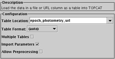
Configuration for Load Table action
The Load Table action takes a URL or filename in the table that points to a table in one of TOPCAT's supported formats, and loads that into TOPCAT as a new table.
Configuration:
(auto) may be used, otherwise the correct format
must be chosen from the list.
<syscmd" or "|syscmd"
syntax described in Section 4.2 may be used to
preprocess the input stream before the table is loaded.
This option is usually not required, and has security implications;
if it is switched on in an action loaded from a session file,
the security panel
will be displayed.
The Plot Table action takes a URL or filename in the table that points to a table in one of TOCAT's supported formats, and displays a plot window that can plot the data from that table. This is like loading the table (e.g. with the Load Table action) and then opening a plot window in the usual way, but doing it this way does not actually load the table into TOPCAT's list of loaded tables, and every time the action is activated, the data from the last invocation is just replaced with that from the current one (as far as possible - the tables need to have a similar structure for each row). In the plot window, the referenced table is listed first in the Table selector (or selectors, if multiple layers are configured) with the special name "0: Activated". All the currently loaded tables are available in the window as well as the activated one, so you can plot those for comparison in the same window if you want.
The configuration of this action lets you select the type of plot window to use, but other than that does not let you specify in detail how you want the plot to look. However, after you have activated the action once, you can interactively configure the plot as required using all the usual plot options, and subsequent activations of the same action will just update the plot with the data from the newly activated row, without affecting the rest of the configuration. This makes it easy to visually compare column data from tables linked in different rows of the original table. Note however that the details of the plot window configuration are not included when a session is saved.
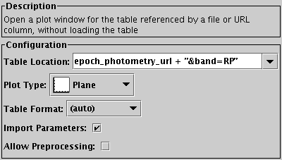
Configuration for Plot Table action
Configuration:
(auto) may be used, otherwise the correct format
must be chosen from the list.
<syscmd" or "|syscmd"
syntax described in Section 4.2 may be used to
preprocess the input stream before the table is loaded.
This option is usually not required, and has security implications;
if it is switched on in an action loaded from a session file,
the security panel
will be displayed.
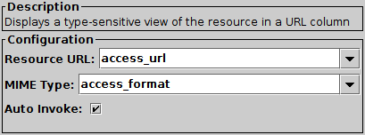
Configuration for View URL action
The View URL activation type uses a URL column and a column giving the MIME type from the activated row, and tries to display the resource in a suitable way for content of the indicated type.
Configuration:
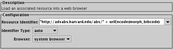
Configuration for View in Web Browser action
The View in Web Browser action uses some kind of location indicator from the activated row and causes it to be displayed in a web browser. If the web page is HTML it should get displayed directly, other content types may get sent to other desktop applications depending on the capabilities and configuration of the browser in use.
In the most straightforward case, the location is a URL supplied by one of the table columns. However TOPCAT knows how to turn various other types of value such as DOIs and filenames into web page addresses, depending on the Identifier Type that's chosen. If none of the identifier types listed below is suitable for you (for instance if you want to use NED with some non-standard options), you can construct your own URL based on column values using the expression language.
Configuration:
2018A&A...616A...2L" turns into
https://ui.adsabs.harvard.edu/abs/2018A%26A...616A...2L.
See the bibcodeUrl
function.
10.3390/informatics4030018" turns into
https://doi.org/10.3390/informatics4030018.
See the doiUrl function.
arXiv:1804.09379" turns into
https://arxiv.org/abs/1804.09381.
See the arxivUrl function.
Beta Pictoris" turns into
https://simbad.cds.unistra.fr/simbad/sim-id?Ident=Beta%20Pictoris.
See the simbadUrl function.
NGC 3952" turns into
http://ned.ipac.caltech.edu/byname?objname=NGC%203952.
See the nedUrl function.
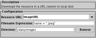
Configuration for Download URL action
The Download URL action uses a URL column or expression defined in the table and downloads its contents to a local file.
Configuration:
name + ".jpeg"
(or equivalently concat(name, ".jpeg"))
takes the content of the name column in the table,
and appends the extension ".jpeg" to make a filename appropriate
for the given row.

Configuration for Delay action
The Delay action just waits for the specified
number of seconds before proceeding.
Any whole or fractional number of seconds can be specified.
It's not much use on its own, but it can be useful in combination
with other actions when preparing a "slide show" with the
Activate All Rows () action.
This action is a convenience;
a similar effect can be achieved using, for instance,
the sleep function in the
Execute Code action.
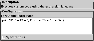
Configuration for Execute Code action
The Execute Code action can execute arbitrary code using the expression language described in Section 7. Most of the expressions and functions just evaluate an expression, and in that case the only effect is that the result of the expression is displayed in the Results panel at the bottom of the activation window every time a row is activated. However, some functions are defined especially for use in this window, and have some additional effect such as popping up a viewer window, writing output to the console, or downloading a file. These are listed below.
In principle, this window can provide very flexible options for defining your own activation actions. In practice, the available activation functions don't give you much more sophisticated options than what is available in the other activation types. However, some more flexible options may be added in the future, and it is also possible to implement your own as explained in Section 7.11. Note that another option for configuring your own custom actions is to use the Run System Command to invoke a shell script or similar with supplied arguments.
Configuration:
The available Activation Functions (ones that have some effect other than just returning a value) are summarised below, and listed in detail in Appendix B.2. You can also browse them interactively in the Activation Functions branch of the Available Functions Window. Note some of these offer rather out of date functionality, and may be withdrawn (replaced by better alternatives) in future releases.
ImageWindow).
Invoking certain activation functions configured by an unknown party has security implications. If this action is loaded from a session file, the security panel will be shown.
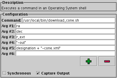
Configuration for Run System Command action
The Run System Command action allows you to invoke an operating system command, for instance running a shell script, when a row is activated, with command parameters taken from table cell values as required.
This functionality has been tested on Unix-like operating systems; it may or may not work well on other OSs (user reports welcome!).
Configuration:
").
The expressions are parsed as they are typed in, and if the current text
of any of the entries does not represent a legal expression,
the action is disabled,
and an error message is displayed in the Status panel
that should help to understand what's wrong.
/)
Executing system commands configured by an unknown party has obvious security implications. If this action is loaded from a session file, the security panel will be shown.
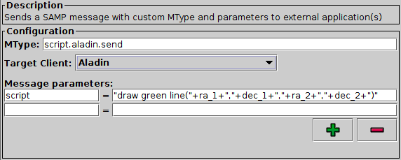
Configuration for SAMP Message action
The SAMP Message action allows you to send a custom SAMP message to other appliacations on the desktop. In most cases it is more straightforward to use one of the standard Send... actions like Send Sky Coordinates, Send FITS Image or Send VOTable, but if you want to send a SAMP message that is not covered by those options, you can use this action instead to control exactly what goes in the message.
To use this action, you need to supply the MType string and (if applicable) name-value pairs for the message parameters. You will of course need to know the MType-specific parameter syntax for the message that you want to send.
Configuration:
/)
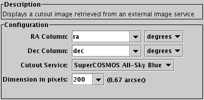
Configuration for Display Cutout Image action
This option presents an easy-to-use way of popping up a cutout image from an image server displaying a region of sky around an activated row. The size of cutout can be selected, and a small selection of image services is provided. When you activate the row, the program will attempt to contact the web server which provides these images, retrieve the image, and display it in one of the internal image viewers.
Note: the list of image services provided by this action is very limited. In most cases, you will be better off using the Display HiPS cutout action.
Configuration:
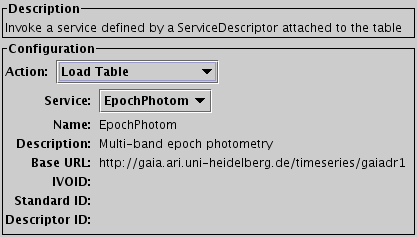
Configuration for Invoke Service action
The Invoke Service action is only appropriate (and only visible by default) for tables in the VOTable (or FITS-plus) format which include Service Desriptor elements as defined in the DataLink standard. These service descriptors can provide information on how to invoke an external data service of some kind, which is usually related to the data in the table, and usually can be invoked differently for each row in the table (for instance using one of the table columns as a parameter of the invocation URL). For instance a Service Descriptor may be attached to a table to provide a rule for finding an additional data product (like a time series or preview image) for each row in a table.
This action invokes one of these service descriptors for the activated row.
Configuration:
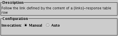
Configuration for Invoke Datalink Row action
The Invoke Datalink Row action is only useful (and only visible by default) for a particular type of table, namely the {links}-response table format defined by the DataLink standard. This format is sometimes loosely known as the DataLink format, and is used to represent links of various kinds to external data resources.
Each row of a DataLink table represents a labelled link to some external resource, and this activation action follows that link in some way when the row is activated, providing options for how it is followed. Note however, that if you have a DataLink table loaded and want to invoke its links, the DataLink Window may provide a more straightforward way to do it than this activation action (the functionality is quite similar to what's here, but fewer popup windows are involved).
Because different rows typically have different kinds of links and so can be invoked in different ways, most of the configuration of link-following behaviour is not done in the Configuration panel of the Activation Window, but in a popup window specific to the row when activation takes place. The per-row popup window, if displayed, has the same content as the lower panel of the DataLink Window. Refer to the documentation of that window for more details.
Configuration:
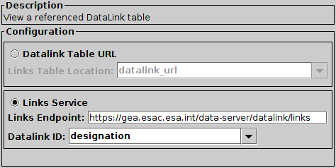
Configuration for View Datalink Table action
The View Datalink Table action is for tables whose rows that can reference files in the {links}-response table format defined by the DataLink standard. Activating a row with this action defined will retrieve the DataLink file from the location indicated and display it in a new popup window. The display is the same as that of the DataLink Window; see the documentation of that window for details. There are a couple of differences however:
There are two alternative ways to configure this action; you can either specify the Datalink Table URL or the Links Service parameters. Select the radio button for one or the other and fill in the details as appropriate.
meta.id" or variants).
Some of the activation actions listed in the previous sections result in popping up windows to view related resources in some way. In many cases, the best thing is to send data to external applications that are optimised for working with different (non-table) data types, but for simple cases TOPCAT provides internal viewers. They are listed in the following subsections.
If you choose the Display Image or Display Cutout Image activation actions, or the View image internally option in one of the DataLink-related actions, TOPCAT will try to display an image in an internal image viewer.
This image viewer is very basic, and looks like this:
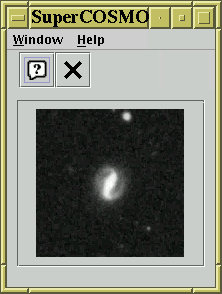
Basic Image Viewer
Alternative options are available to communicate with external image viewers.
Note: earlier versions of TOPCAT offered a more capable image viewer called SoG under some circumstances. However, this only worked when the Java Advanced Imaging classes were present at runtime, and these are hard to obtain now, so this option has been withdrawn.
If you try to display a spectrum internally, TOPCAT may be able to pop up a SPLAT sub-window.
SPLAT is a sophisticated multi-spectrum analysis program. This requires the presence of a component named JNIAST, which may or may not have been installed with TOPCAT (it depends on some non-Java, i.e. platform-specific code). There is currently no fallback spectrum viewer, so if JNIAST is not present, then spectra cannot be displayed internally. An example of SPLAT display of multiple spectra is shown below.
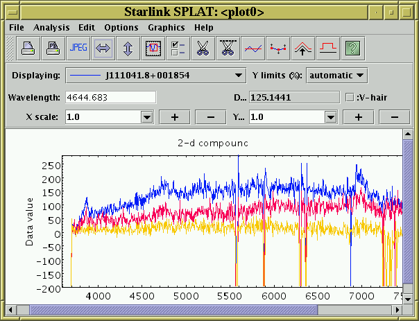
SPLAT Spectrum Viewer
Full documentation for SPLAT is available on-line within the program, or in SUN/243.
In general it is more reliable and configurable to use SAMP to send spectra to an external running instance of SPLAT, via the Send Spectrum action.
If you choose the View in Web Browser action then activating a row will display the web page whose URL is in one of the columns in a web browser. You are given the option of what browser you would like to use in this case; the options available depend on your java installation.
The Basic Browser and JavaFX Browser options use an internal browser implementation that runs inside the TOPCAT application itself. This can view HTML or plain text pages and has forward and back buttons which work as you'd expect. The JavaFX variant has more capabilities and generally works better, for instance it can render JavaScript as well as static HTML, so it's generally better to select this if it's available, but it's not present in all Java Runtime Environments. The Basic variant is always available. These browsers look approximately like this:
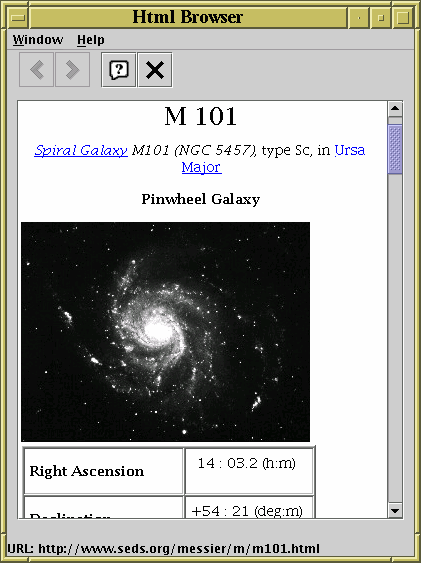
Basic HTML browser
Alternatively, the System Browser option may be available. This will send the URL to the default browser installed on your desktop. This will certainly be a more capable browser implementation than the internal options, but there may be annoyances; for instance in some cases it opens a new tab every time a new URL is opened.
Activation actions can be configured to perform a wide variety of user-defined actions, in some cases including actions that could have damaging consequences. For instance the Run System Command action can execute arbitrary system (shell) commands with the permissions of the user running the TOPCAT application. As long as the TOPCAT user is the person who has configured these commands, this is no more dangerous than the same user sitting down at the keyboard to type shell commands.
In the case of Activation Actions that have been loaded from a Session file however, it is possible that the person who saved the session might have configured it to perform malicious actions affecting whoever re-loads it. TOPCAT can't determine whether an action is actually malicious, but it can identify actions which could be configured to do malicious things. In the case that it detects an Activation Action that has been loaded from a Session file that might be doing something dangerous (invoking arbitrary system commands, or in general anything that has effects outside of the TOPCAT application itself, excepting some known-harmless SAMP messages) it will ask the user for explicit approval before invoking it.
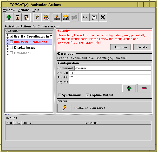
Activation Window configured with security implications
This screenshot shows what happens. When called upon to invoke a potentially dangerous pre-configured action, it displays the Security panel in red, and the user has to click the Approve button before the action will be invoked. If you see this, you should, as instructed, check that the action configuration is not doing anything it shouldn't. Once you have approved it, the security panel will disappear and later invocations will take place with no further user interaction.
If you know that the session file is harmless, and you don't
want to be bothered by these approval messages, you can use the
Approve All Actions () menu item
in the Actions menu.
The Run System Command
and Execute Code
actions can trigger these warnings for fairly obvious reasons.
They can however also be triggered under some circumstances by
Display Image,
Load Table and
Plot Table.
That's because in some configurations these actions can allow
file/URL location values that perform preprocessing of the input streams
using the "<syscmd" or "syscmd|" syntax
described in Section 4.2, and that means that referencing
image/table locations either entered directly, or acquired from table data,
could result in execution of arbitrary system commands.
This preprocessing is always switched off by default,
and you shouldn't switch it on unless you need it,
so it will not apply unless you have turned it on explicitly or
loaded it from a session file.
In nearly all cases, you don't need to think about these issues, but if you are loading a session file that may have been prepared by somebody else, TOPCAT will warn you in case anything malicious might be capable of affecting you.
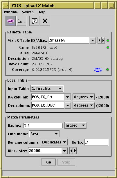
CDS Upload X-Match Window
The CDS Upload X-Match Window allows you to join a local table
with any table provided by the
VizieR
database of astronomical tables or with
SIMBAD.
You can access the window from the main
Control Window using the
CDS Upload Match button ()
in the toolbar, or the Joins or VO menus.
This window is an interface to the excellent
CDS X-Match service
provided by the Centre de Données astronomiques de Strasbourg
(CDS).
The service is very fast, and in most cases it is the best way to
match a local table against a large external table hosted by a service.
In particular, it is almost certainly much better than using
the Multi-Cone window,
though it's less flexible than TAP.
The local table is uploaded to the X-Match service in blocks, and the matches for each block are retrieved in turn and eventually stitched together to form the final result. The tool only uploads sky position and an identifier for each row of the input table, but all columns of the input table are reinstated in the result for reference. These details are mostly transparent when using the service, though it may help to understand how the progress bar moves.
For a better understanding of the details of how this service operates, including exactly what coordinates are matched against the uploaded positions (roughly: integrated to J2000 using proper motions if available) and what columns are included in the output (roughly: a subset of the most commonly used columns), please consult the service documentation. Note that because of the way the service is implemented not all the columns from the VizieR table may be present in the result; if the columns you need are not present, you're out of luck, there's no way to request additional ones.
The window has three panels, described below.
The Remote Table panel allows you to select the CDS table against which to match. The table must be entered by name in the VizieR Table ID/Alias field, and may be in one of the following forms:
When a table name has been entered, additional information (Name, Alias, Description and Row Count) will be downloaded from CDS and displayed in the lower part of the Remote Table panel. If nothing shows up here, then the table name is not legal for the X-Match service, and the Go button will be disabled.
Sky coverage information is also displayed, including the proportion of the sky covered by the table and a graphical indication of the covered regions on the sky.
Service interaction is monitored by the little "lights" to the right of this panel. If things are operating correctly they should be, or quickly turn, green. If they are amber or red, the service may be slow or not responding. Hovering over them with the mouse will give more information (apologies to red-green colourblind users).
The Local Table panel allows you to indicate the local table (the one loaded into TOPCAT) that you want to match. You must select the required table and indicate its Right Ascension and Declination columns.
The Match Parameters panel supplies the other information about how the match will operate:
Large blocksizes tend to be good (up to a point) for reducing the total amount of time a large xmatch operation takes, but they can make it harder to see the job progressing. There is also the danger (for ALL-type find modes) of exceeding the return size limit, which will result in truncation of the returned result. If this happens, a warning will be included in the popup window that reports match completion. At time of writing, the upload limit is 100Mbyte (about 3Mrow), and the maximum return size is 2Mrow.
When all the fields have been filled in, hit the Go button and the match will start; progress will be logged in the progress bar at the bottom of the window. To stop the match before it has completed, hit the Stop button. Note that the Go button is only enabled when a legal table name has been entered at the top.
The remote table in most cases contains only a subset of the the columns in the relevant VizieR table, including the most useful ones. The service currently provides no straightforward way to acquire columns which are not returned by default.
The following item is available in the toolbar and Search menu:
Use Service Coverage
Acknowledgement: CDS note that if the use of the X-Match service is useful to your research, they would appreciate the following acknowledgement:
"This research made use of the cross-match service provided by CDS, Strasbourg."
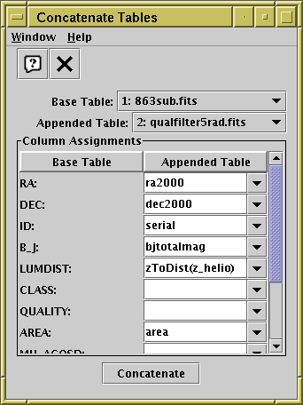
Concatenation Window
The Concatenation Window allows you to join two tables together
top-to-bottom. It can be obtained using the
Concatenate Tables item () in the
Control Window Joins menu.
When two windows are concatenated all the rows of the first ("base") table are followed by all the rows of the second ("appended") table. The result is a new table which has a number of rows equal to the sum of the two it has been made from. The columns in the resulting table are the same as those of the base table. To perform the concatenation, you have to specify which columns from the appended table correspond to which ones in the base table. Of course, this sort of operation only makes sense if at least some of the columns in both tables have the same meaning. This process is discussed in more detail in Section 5.1.
The concatenation window allows you to select the base and appended tables, and for each column in the base table to specify what quantity in the appended table corresponds to it. You can either select a column from the appended table from the selection box, or type in an expression in the expression language referring to columns from the appended table. If you leave the field blank, the column in question will have all null entries in the resulting table. Only suitable columns are available for choosing from these column selectors, that is ones matching the data type of the base column.
In some cases these column selectors may have a value filled in automatically if the program thinks it can guess appropriate ones, but you should ensure that it has guessed correctly in this case. If the two tables have essentially the same structure, the corresponding columns should all get filled in automatically.
When you have filled in the fields to your satisfaction, hit the Concatenate button at the bottom of the window, and a new table will be created and added to the table list in the Control Window (a popup window will inform you this has happened).
The result is created from the Apparent versions of the base and appended tables, so that any row subsets, hidden columns, or sorts currently in force will be reflected in the output.
The SAMP Window displays the status of SAMP messaging and allows some
control over its configuration.
You can display it using the SAMP Status item ()
in the Control Window
Interop menu or toolbar.
SAMP is a messaging protocol which
allows TOPCAT to exchange information with other desktop applications -
see Section 9 for details.
The main part of the window is a tabbed panel which displays the status of the SAMP connection in detail.
The first tab is labelled Clients:
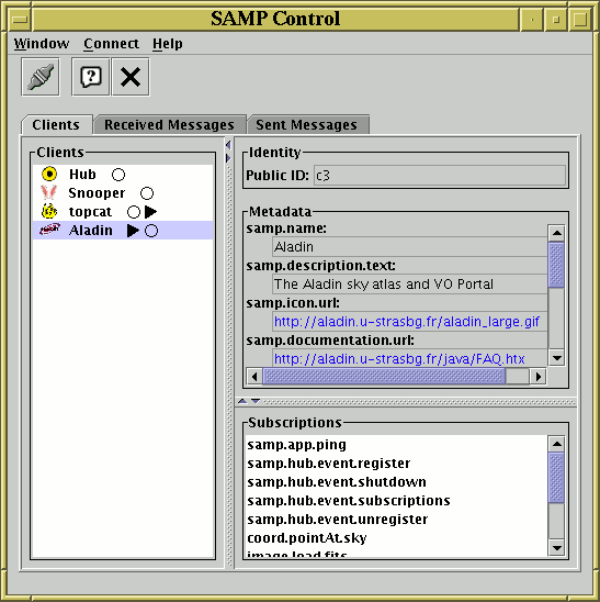
SAMP Window Clients tab
This displays details of all applications (including TOPCAT itself) which are currently registered with the hub. If you select a client in the list on the left hand side of the panel, you will see its details on the right hand side. This includes its Metadata (which may include things like its name, author, documentation URL etc) and its Subscriptions which describes what types of messages (MTypes) it will respond to. Also in the list on the left is for each application a graphical indication of messages recently received by/sent from it, in which TOPCAT is the other partner. These are represented by little arrows before/after the little circle following the application name. In the figure, a message is currently in progress from TOPCAT to Aladin. More detail on this is shown in the other tabs.
The other two tabs are labelled Received Messages and Sent Messages. They look very similar to each other:
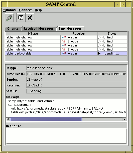
SAMP Window Sent Messages tab
They display details of SAMP messages recently sent from or received by TOPCAT. A table near the top contains one row for each message. Shown in different columns are the message's MType (which describes the message semantics), the application receiving/sending it from/to TOPCAT, and a summary of its status. If you click on the row, all the details of the message, including its content and that of the response if one has been received, are visible in the lower panel. Messages remain in this table for a few seconds after they have completed, but are eventually removed to avoid clutter.
The following toolbar button is available:
 Connect/Disconnect
If no hub is running, clicking this button will pop up a dialogue box which allows you to start a hub. You are given the option to start either an internal or an external hub. An internal one runs in the same Java Virtual Machine as TOPCAT itself, and an external one runs in a separate process. The main important difference is that an internal hub will shut down when TOPCAT does, while an external hub will keep running until it is shut down explicitly. If an external hub is started, a window which shows its status is displayed on the screen; closing this window (which does not belong to TOPCAT) will shut down the hub.
More facilities may be introduced into this window in future releases.
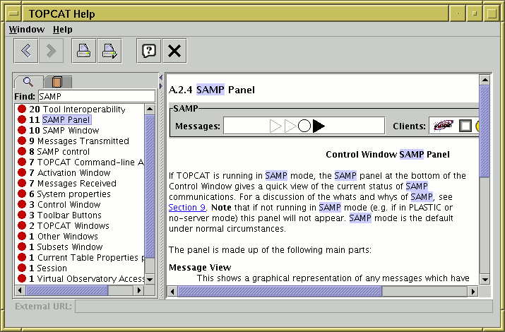
Help Window
The help window is a browser for displaying help information on TOPCAT;
it can be obtained by clicking the Help () button
that appears in the toolbar of most windows.
It views the text contained in this document, so it may be what you are
looking at now.
The panel on the right hand side displays the currently selected section of help text itself. The panel on the left gives a couple of ways of selecting this view:
 Text Search
 Table of Contents
The bar in between the two panels can be dragged with the mouse to affect the relative sizes of these windows.
The toolbar contains these extra buttons:
 Back
Back
 Forward
Print
Forward
Print
 Page Setup
 To Browser
Although the printing buttons work, if you want to print out the
whole of this document rather than just a few sections you may be better off
printing the PDF version,
or printing the single-page HTML version through a web browser.
The most recent version of these should be available
on the web at
http://www.starlink.ac.uk/topcat/sun253/sun253.html and
http://www.starlink.ac.uk/topcat/sun253.pdf;
you can also find the HTML version in the topcat jar file at
uk/ac/starlink/topcat/help/sun253.html
or, if you have a full TOPCAT installation, in
docs/topcat/sun253/sun253.html and
docs/topcat/sun253.pdf
(the single-page HTML version is available
here in the HTML version).
The help browser is an HTML browser and some of the hyperlinks in the help document point to locations outside of the help document itself. Selecting these links will go to the external documents. When the viewer is displaying an external document, its URL will be displayed in a line at the bottom of the window. You can cut and paste from this using your platform's usual mechanisms for this.
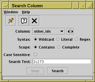
Column Search window
The Column Search window lets you search through the values
in a chosen column of the displayed JTable
to find occurrences of some particular text.
It is currently available from the
Data Window and
Columns Window.
In each case you can get it by using the
Search Column () action in one of two ways:
either click the toolbar button or menu item,
in which case you have to choose the column of interest using the selector,
or select it from the popup menu that appears when you right-click
on a column, in which case that column is selected automatically.
To perform a search, ensure that the column selector is filled in
with the column you want to search,
fill in the matching options,
enter the text to search for,
and hit the Search button.
Any rows matching the query are then highlighted in the
corresponding JTable,
and the display is scrolled so that the first match, if any, is visible.
If at least one match is found, the search window usually closes
(though this can be prevented with the
Stay Open () option).
When used with the Data Window only, if exactly one matching row was found, it is also activated. You can see how many matches there were from the Selected value indicated at the bottom of the Data Window.
The fields to fill in are as follows:
*" matches any sequence of characters, and
"?" matches any single characterThe Search button will only be enabled if the controls specify a legal search condition. If for instance the search text is empty, or Regex syntax is chosen and the search text is not a legal regular expression, it will be disabled.
The search will usually complete straight away, but if the table is very long it may take a significant amount of time. In this case progress is displayed with the progress bar at the bottom of the window, and you can interrupt the running search using the Stop button.
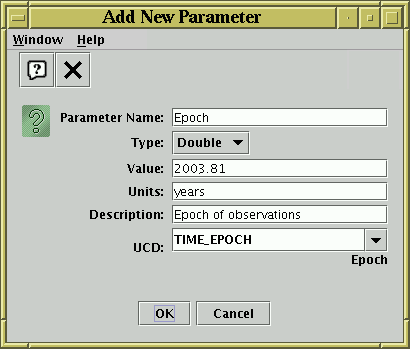
New Parameter dialogue window
The New Parameter window allows you to enter a new table parameter
to be added to a table.
It can be obtained by clicking the New Parameter ()
button in the Appendix A.3.2.
A parameter is simply a fixed value attached to a table and can contain
information which is a string, a scalar, an array... in fact exactly
the same sorts of values which can appear in table cells.
The window is pretty straightforward to use: fill in the fields and click OK to complete the addition. The Type selector allows you to select what kind of value you have input. The only compulsory field is Parameter Name; any of the others may be left blank, though you will usually want to fill in at least the Value field as well. Often, the parameter will have a string value, in which case the Units field is not very relevant.
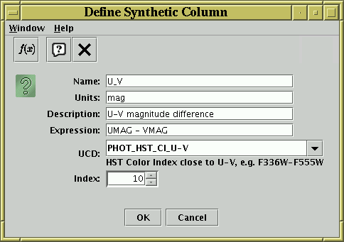
Synthetic Column dialogue window
The Synthetic Column Window allows you to define a new "Synthetic" column,
that is one whose values are defined using an algebraic expression
based on the values of other columns in the same row.
The idea is that the value of the cells in a given row in this column
will be calculated on demand as a function of the values of cells
of other columns in that row. You can think of this as providing
functionality like that of a column-oriented spreadsheet.
You can activate the dialogue using the
Add Column () or
Replace Column () buttons in the
Columns Window or from the
(right-click) popup menu in the Data Window.
The window consists of a number of fields you must fill in to define the new column:
) button on the toolbar.
pos.eq.ra) which may help.
Note however that UCDs can be composed by assembling multiple words
(e.g. pos.eq.ra;meta.main), so the selection list is
not exhaustive. You can type any text into the field.
Having filled in the form to your satisfaction, hit the OK button at the bottom and the new column will be added to the table. If you have made some mistake in filling in the fields, a popup window will give you a message describing the problem. This message may be a bit arcane - try not to panic and see if you can rephrase the expression in a way that the parser might be happier with. If you can't work out the problem, it's time to consult your friendly local Java programmer (failing that, your friendly local C programmer may be able to help) or, by all means, contact the author.
If you wish to add more metadata items you can edit the appropriate cells in the Columns Window. You can edit the expression of an existing synthetic column in the same way.
Once created, a synthetic column is added to the Apparent Table and behaves just like any other; it can be moved, hidden/revealed, used in expressions for other synthetic columns and so on. If the table is saved the new column and its contents will be written to the new output table.
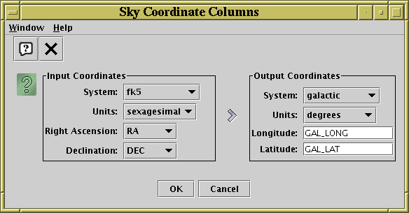
Sky Coordinates Window
The Sky Coordinates Window allows you to add new columns to a table,
representing coordinates in a chosen sky coordinate system.
The table must already contain columns which represent sky coordinates;
by describing the systems of the existing and of the new coordinates,
you provide enough information to calculate the values in the new columns.
You can activate this dialogue using the
New Sky Coordinate Columns () button
in the Columns Window.
The dialogue window has two halves; on the left you give the existing columns which represent sky coordinates, their coordinate system (ICRS, fk5, fk4, galactic, supergalactic or ecliptic) and the units (degrees, radians or sexagesimal) that they are in. Note that the columns available for selection will depend on the units you have selected; for degrees or radians only numeric columns will be selectable, while for sexagesimal (dms/hms) units only string columns will be selectable. On the right you make the coordinate system and units selections as before, but enter the names of the new columns in the text fields. Then just hit the OK button, and the columns resulting from the coordinate conversion will be appended at the right of the table.
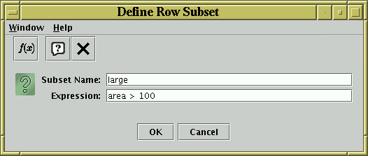
Algebraic Subset dialogue window
The Algebraic Subset Window allows you to define a new
Row Subset which uses an algebraic expression
to define which rows are included. The expression must be a
boolean one, i.e. its value is either true or false for each row of
the table.
You can activate this dialogue using the
Add Subset () button in the
Subsets Window.
The window consists of two fields which must be filled in to define the new subset:
) button on the toolbar.
Having filled in the form to your satisfaction, hit the OK button at the bottom and the new subset will be added to the list that can be seen in the Subsets Window where it behaves like any other. If you have made some mistake in filling in the fields, a popup window will give you a message describing the problem.
The Multi Algebraic Subset Window is displayed when an action
can create more than one subset with algebraic definitions at once.
This happens on completion of the
Draw Algebraic Subset () or
Algebraic Subset From Visible ()
actions;
more than one subset may result if more than one data set is plotted.
If there is more than one subset to be added, they will be shown here
in separate rows.
Often however, only one subset will be presented.
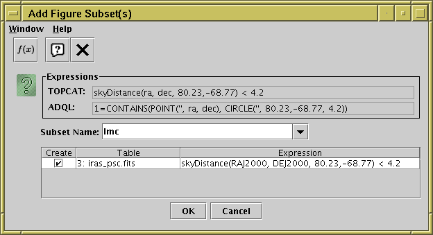
Multi Algebraic Subset Window showing a subset expression to add
The Subset Name selector gives the name of the subset that will be added. You can type in a new name, or select one from the list of existing subsets if you wish to redefine one (re-use an existing subset name). Note: if you re-use an existing name, the expression must not reference that name directly or indirectly. If it does, an error will be displayed, and you will have to choose again.
Each row has the following entries:
Once you are happy with the configuration, hit the OK button and the subset(s) will be created.
An Expressions panel also appears
at the top of the window.
This will, if possible, show representations of the selected region:
TOPCAT uses the expression
language used elsewhere in the application, and
ADQL uses ADQL syntax.
The ADQL form can be cut and pasted for use in the WHERE clause
of a query in the TAP window.
The variable names in these expressions are generic
(e.g. "x" and "y" for Cartesian axes),
instead of the actual quantities plotted, which are used in the subset
expressions below.
Note: the display of expression information in this window is somewhat experimental; better support for region descriptions may be provided elsewhere in the application in some future release.
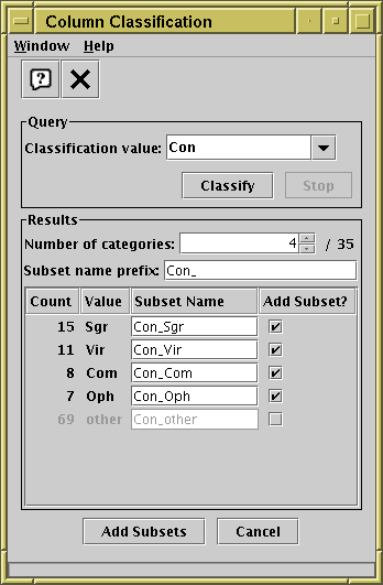
Column Classification Window
The Column Classification Window takes a column or other algebraic expression, and generates a number of mutually exclusive Row Subsets based on its contents. For instance if you have a column with different integer values representing different object types, this window will let you add a new subset to the table for each of the distinct values (object types) appearing in the table. Each subset contains rows with a single value of the classification expression you supply. In the above example, a new subset will be created for each of the four most commonly-occurring constellations in the table.
You can activate this dialogue using the
Classify By Column () button in the
Subsets Window.
In the Query panel, you specify the
expression you want to classify on.
You can select a simple column name from the drop-down list,
or type in an algebraic expression as described in Section 7.
If you want to classify on ranges of values rather than exact
equivalence you can use an expression that rounds to an integer,
for instance "toInteger(RMAG/2.0)*2" would give you subsets
corresponding to bins of width 2 in magnitude.
When you have entered the expression, you may need to click the
Classify button to start the classification
(or it may happen automatically).
The classification will often complete straight away,
but for large tables it could take a noticeable amount of time,
in which case a progress bar is shown at the bottom of the window.
You can stop a long-running classification in progress with the
Stop button.
If you have a very large table with many distinct categories in the given
column, the process can take a lot of memory - if the application runs out
of memory, a warning will pop up and the classification will not complete.
When the classification has run, the results are displayed in the Results panel. Two fields control the way these results are displayed:
The results are displayed in a table, each row corresponding to a Row Subset that can be added to the table based on the classification. The subsets are shown in decreasing order of popularity (the subset containing the most rows is listed first). The final row, labelled "other", groups all the rows which are not in any of the other currently selected and displayed subsets. The following columns are shown:
When you have adjusted subset names and selected the ones you want to add, click the Add Subsets button at the bottom, and one subset will be added to the table for each of the items with the Add Subset? checkbox ticked. If you don't want to add any of these subsets after all, just hit Cancel or close the window.
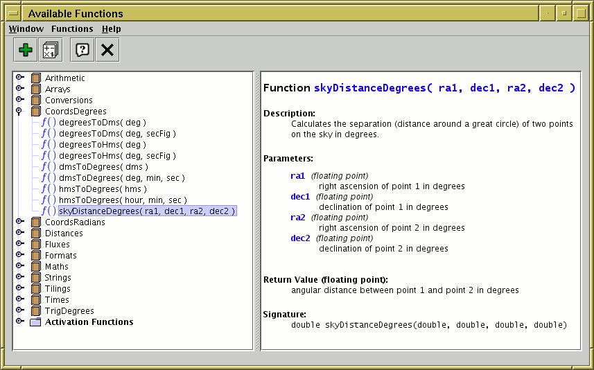
Available Functions Window
This window displays all the functions (Java methods) which are
available for use when writing
algebraic expressions.
This includes both the built-in expressions and any
extended ones you might have added.
You can find this window by using the
Show Functions () button in the
Synthetic Column or
Algebraic Subset
window toolbars.
On the left hand side of the window is a tree-like representation of the functions you can use. Each item in this tree is one of the following:
 Folder
 Class
Class
 Function
 Constant
Of these, the Folder and Class items have a 'handle' (),
which means that they contain other items
(classes and functions/constants respectively).
By clicking on the handle (or equivalently double-clicking on the name)
you can toggle whether the item is open (so you can see its contents)
or closed (so you can't). So to see the functions in a class,
click on its handle and they will be revealed.
You can click on any of these items and information about it
will appear in the right hand panel. In the case of functions
this describes the function, its arguments, what it does, and
how to use it. The explanations should be fairly self-explanatory;
for instance the description in the figure above indicates that
you could use the invocation skyDistanceDegrees(RA1,DEC1,RA2,DEC2)
as the expression for a new table column which gives the angular distance
between two sky positions represented by columns with the names RA1, DEC1
and RA2, DEC2.
Examples of a number of these functions are given in
Section 7.10.
There are two menu/toolbar actions:
 Syntax Help
Add Class
Syntax Help
Add Class
jel.classes or
jel.classes.activation at startup,
as described in Section 7.11.
Classes added either using the Add Class action above or
the jel.classes or jel.classes.activation
system properties will be visible in the tree in this window,
but they may not have proper documentation
(clicking on them may not reveal a description in the right hand panel).
This window displays global variables
and allows you to adjust their values.
You can find it by using the Global Variables
() toolbar button
in the main Control Window
or the equivalent menu option in its File menu.
The variables controlled here can be used in the expression language, for instance when defining new synthetic columns and subsets, or in column selectors such as those used for plot coordinates, or for the function expression in function plots. Adjusting the values of the variables in this window will then have an instant effect on the columns, subsets and plots that depend on them.
This can allow you for instance to experiment with aspects of a
plot such as subset inclusion or coordinate definitions by
changing variable values using the slider in this window
and seeing how plots dependent on the variable in question change.
There is one caveat to this: if visible plots dependent on a variable
being changed in this way are very large or numerous,
such adjustments can result in a lot of computation or I/O and slow
things down.
The plot windows therefore have a
Replot on Data Change () button
that allow you to prevent such immediate updates, which will then
only take place on a replot which is triggered in some other way.
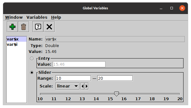
Variables Window
The window is in two parts.
On the left is a list of the currently defined variables.
By default there are two of these:
var$x is a floating point variable, and
var$i is an integer variable,
but new ones can be added.
Selecting one of the names in the list by clicking on it
shows the corresponding value panel on the right.
The right hand panel lets you adjust the selected variable's value. Its appearance differs slightly depending on whether the variable is floating point or integer. There are two ways to change the value, the Entry and the Slider controls. Only one of these is active at a time, use the radio buttons on the left to choose which one to use.
In the case of integer variables, there are also +1/-1 buttons that will nudge the value up and down by 1.
In the case of floating point variables, there is also a Scale selector that lets you choose the scaling between the lower and upper slider bounds to one of the available scaling options (linear, log, asinh and symlog). Since some of these options (logarithmic) require positive definite values, changing the scaling may force a reset of the range values.
The following toolbar/menu items are available:
Add new variable
$ and _,
other characters alphanumeric).
Any unused name matching that constraint is allowed,
but beware of choosing names that may clash with other terms
in the expression language such as column or subset names.
Sticking to the var$xxx convention is a good way
to prevent that happening.
Remove selected variable
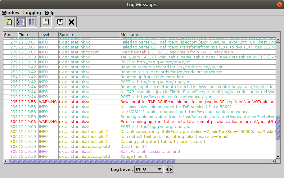
Log Window
The log window can be obtained using the
View Log ()
option on the File menu of the
Control Window.
This window displays any log messages which the application has
generated.
These messages are not required reading for users, but they can be
useful for debugging in case of problems,
and they can also tell you some useful information about what
the application is doing, for instance external URLs that are being
accessed or ADQL query text.
These messages can be useful if you want to reproduce some parts of
TOPCAT's behaviour outside the application, e.g. using curl
or a web browser.
The messages are colour-coded to some extent. WARNING- and SEVERE-level messages, which generally indicate some kind of problem that may cause trouble, are displayed in red and black respectively. INFO- and CONFIG-level messages, which generally just provide information about what's going on under the hood, are assigned an arbitrary colour based on the code subsystem (the Source value) that has generated them. These colours are not really significant, they are just intended as a visual aid.
The Level selector at the bottom can be used as a filter so that only messages beyond a certain severity are displayed.
Depending on whether the -verbose flag
has been specified,
some or all of the displayed messages may have been written
to the console as well
(if there is a console - this depends on how you have invoked TOPCAT).
There is a limit (currently 1000) to the number of logging messages retained, so for long-running instances the older ones may be discarded.
The following toolbar/menu items are available:
 Clear
Clear
 Auto-scroll
 Pause logging
Export to file
Pause logging
Export to file
Note: the messages displayed here are those written through Java's
logging system.
Although it tries not to disturb things too much, TOPCAT's
manipulation of the logging infrastructure affects how it is
set up, so if you have customised your logging setup using,
e.g., the java.util.logging.config.* system
properties, you may find that it's not behaving exactly as
you expected. Sorry.
This appendix lists the functions which can be used in algebraic expressions (see Section 7). They are listed in two sections: the first gives the functions available for use anywhere an expression can be used, and the second gives those only for use in defining custom Activation Actions.
This information is also available within TOPCAT from the
Available Functions Window,
obtained using the toolbar button.
The following functions can be used anywhere that you can write an algebraic expression in TOPCAT. They will typically be used for defining new synthetic columns or algebraically-defined row subsets. The documentation in the following subsections is also available from within TOPCAT in the Available Functions Window.
Standard arithmetic functions including things like rounding, sign manipulation, and maximum/minimum functions. Phase folding operations, and a convenient form of the modulus operation on which they are based, are also provided.
roundUp( x )
x (floating point): a value.x rounded uproundDown( x )
x (floating point): a valuex rounded downround( x )
x (floating point): a floating point value.x rounded to the nearest integerroundDecimal( x, dp )
float (32-bit floating point value),
so this is only suitable for relatively low-precision values.
It's intended for truncating the number of apparent significant
figures represented by a value which you know has been obtained
by combining other values of limited precision.
For more control, see the functions in the Formats class.
x (floating point): a floating point valuedp (integer): number of decimal places (digits after the decimal point)
to retainx but with a
limited apparent precisionroundDecimal(PI,2) = 3.14f
abs( x )
x (integer): the argument whose absolute value is to be determinedabs( x )
x (floating point): the argument whose absolute value is to be determinedmax( a, b )
Multiple-argument maximum functions are also provided in the
Arrays and Lists packages.
a (integer): an argument.b (integer): another argument.a and b.maxNaN( a, b )
a (floating point): an argument.b (floating point): another argument.a and b.maxReal( a, b )
Multiple-argument maximum functions are also provided in the
Arrays and Lists packages.
a (floating point): an argumentb (floating point): another argumenta and b
min( a, b )
Multiple-argument minimum functions are also provided in the
Arrays and Lists packages.
a (integer): an argument.b (integer): another argument.a and b.minNaN( a, b )
a (floating point): an argument.b (floating point): another argument.a and b.minReal( a, b )
Multiple-argument minimum functions are also provided in the
Arrays and Lists packages.
a (floating point): an argumentb (floating point): another argumenta and b
mod( a, b )
a/b.
This is a modulo operation, but differs from the expression
a%b in that the answer is always >=0
(as long as b is not zero).
a (floating point): dividendb (floating point): divisora by b
modulo(14, 5) = 4
modulo(-14, 5) = 1
modulo(2.75, 0.5) = 0.25
phase( t, period )
For positive period, the returned value is in the range [0,1).
t (floating point): valueperiod (floating point): folding periodphase(7, 4) = 0.75
phase(-1000.5, 2.5) = 0.8
phase(-3300, 33) = 0
phase( t, period, t0 )
t0 corresponds to phase zero.
For positive period, the returned value is in the range [0,1).
t (floating point): valueperiod (floating point): folding periodt0 (floating point): reference value, corresponding to phase zerophase(5003,100,0) = 0.03
phase(5003,100,2) = 0.01
phase(5003,100,4) = 0.99
phase( t, period, t0, phase0 )
t0 corresponds to integer phase
value, and the phase offset phase0 determines the
starting value for the phase range.
For positive period, the returned value is in the range
[phase0,phase0+1).
t (floating point): valueperiod (floating point): folding periodt0 (floating point): reference value, corresponding to phase zerophase0 (floating point): offset for phasephase(23,10,1,99) = 99.2
phase(8.6125,0.2,0.0125,-0.3) = 0
phase(8.6125,0.2,0.1125,-0.7) = -0.5
Functions which operate on array-valued cells. The array parameters of these functions can only be used on values which are already arrays (usually, numeric arrays). In most cases that means on values in table columns which are declared as array-valued. FITS and VOTable tables can have columns which contain array values, but other formats such as CSV cannot.
If you want to calculate aggregating functions like sum, min, max etc
on multiple values which are not part of an array,
it's easier to use the functions from the Lists class.
Note that none of these functions will calculate statistical functions over a whole column of a table.
The functions fall into a number of categories:
size,
count,
countTrue,
maximum,
minimum,
sum,
mean,
median,
quantile,
stdev,
variance,
join.
add,
subtract,
multiply,
divide,
reciprocal,
condition,
slice,
pick.
Mostly these work on any numeric array type and return
floating point (double precision) values,
but some of them (slice, pick)
have variants for different array types.
array,
which lets you assemble a floating point array value from
a list of scalar numbers.
There are variants (intArray, stringArray)
for some different array types.
sum( array )
array is not a numeric array, null
is returned.
array (Object): array of numbersarray
mean( array )
array is not a numeric array, null
is returned.
array (Object): array of numbersarray
variance( array )
array is not a numeric array,
null is returned.
array (Object): array of numbersarray
stdev( array )
array is not a numeric array,
null is returned.
array (Object): array of numbersarray
minimum( array )
array is not a numeric array, null
is returned.
array (Object): array of numbersarray
maximum( array )
array is not a numeric array, null
is returned.
array (Object): array of numbersarray
median( array )
array is not a numeric array, null
is returned.
array (Object): array of numbersarray
quantile( array, quant )
quant value;
values of 0, 0.5 and 1 give the minimum, median and maximum
respectively. A value of 0.99 would give the 99th percentile.
array (Object): array of numbersquant (floating point): number in the range 0-1 deterining which quantile
to calculatequant
size( array )
array is not an array, zero is returned.
array (Object): arrayarray
count( array )
array is not an array, zero is returned.
array (Object): array (may or may not be numeric)array
countTrue( array )
array (array of boolean): array of true/false valuesarray
join( array, joiner )
array is not an array, null is returned.
array (Object): array of numbers or stringsjoiner (String): text string to interpose between adjacent elementsarray elements separated by
joiner stringsjoin(array(1.5,2.1,-3.9), "; ") = "1.5; 2.1; -3.9"
dotProduct( array1, array2 )
array1 (Object): first arrayarray2 (Object): second arraydotProduct(array(3,4,5), array(1,2,3)) = 26
add( arrayOrScalar1, arrayOrScalar2 )
If the arguments are not as expected (e.g. arrays of different lengths, both scalars, not numeric) then null is returned.
arrayOrScalar1 (Object): first numeric array/scalararrayOrScalar2 (Object): second numeric array/scalararrayOrScalar1 + arrayOrScalar2,
the same length as the input array(s)add(array(1,2,3), array(0.1,0.2,0.3))
= [1.1, 2.2, 3.3]
add(array(1,2,3), 10) = [11,12,13]
subtract( arrayOrScalar1, arrayOrScalar2 )
If the arguments are not as expected (e.g. arrays of different lengths, both scalars, not numeric) then null is returned.
arrayOrScalar1 (Object): first numeric array/scalararrayOrScalar2 (Object): second numeric array/scalararrayOrScalar1 - arrayOrScalar2,
the same length as the input array(s)subtract(array(1,2,3), array(0.1,0.2,0.3))
= [0.9, 1.8, 2.7]
subtract(array(1,2,3), 1.0)
                 = [0, 1, 2]
multiply( arrayOrScalar1, arrayOrScalar2 )
If the arguments are not as expected (e.g. arrays of different lengths, both scalars, not numeric) then null is returned.
arrayOrScalar1 (Object): first numeric array/scalararrayOrScalar2 (Object): second numeric array/scalararrayOrScalar1 * arrayOrScalar2,
the same length as the input array(s)multiply(array(1,2,3), array(2,4,6)) = [2, 8, 18]
multiply(2, array(1,2,3)) = [2, 4, 6]
divide( arrayOrScalar1, arrayOrScalar2 )
If the arguments are not as expected (e.g. arrays of different lengths, both scalars, not numeric) then null is returned.
arrayOrScalar1 (Object): first numeric array/scalararrayOrScalar2 (Object): second numeric array/scalararrayOrScalar1 / arrayOrScalar2,
the same length as the input array(s)divide(array(0,9,4), array(1,3,8)) = [0, 3, 0.5]
divide(array(50,60,70), 10) = [5, 6, 7]
reciprocal( array )
array argument is not a numeric array,
null is returned.
array (Object): array inputarray parameterreciprocal(array(1,2,0.25) = [1, 0.5, 4]
condition( flagArray, trueValue, falseValue )
This has the same effect as applying the expression
outArray[i] = flagArray[i] ? trueValue : falseValue.
flagArray (array of boolean): array of boolean valuestrueValue (floating point): output value corresponding to an input true valuefalseValue (floating point): output value corresponding to an input false valueflagArray
condition([true, false, true], 1, 0) = [1, 0, 1]
constant( n, value )
Note:
This documents the double-precision version of the routine.
Corresponding routines exist for other data types
(float, long, int,
short, byte).
n (integer): size of output arrayvalue (floating point): value of every element in the output arrayn-element array with every element set to
value
constant(5, 23.5) = [23.5, 23.5, 23.5, 23.5, 23.5]
slice( array, i0, i1 )
The semantics are like python array slicing, though both limits
have to be specified: the output array contains the sequence of
elements in the input array from i0 (inclusive)
to i1 (exclusive). If a negative value is given
in either case, it is added to the length of the input array,
so that -1 indicates the last element of the input array.
The indices are capped at 0 and the input array length respectively,
so a large positive value may be used to indicate the end of the array.
If the end index is less than or equal to the start index,
a zero-length array is returned.
Note:
This documents the double-precision version of the routine.
Corresponding routines exist for other data types
(float, long, int,
short, byte, String,
Object).
array (array of floating point): input arrayi0 (integer): index of first element, inclusive
(may be negative to count back from the end)i1 (integer): index of the last element, exclusive
(may be negative to count back from the end)i0 and i1
slice(array(10,11,12,13), 0, 3) = [10, 11, 12]
slice(array(10,11,12,13), -2, 999) = [12, 13]
pick( array, indices, ... )
The output array consists of one element selected from the input array for each of the supplied index values. If a negative value is supplied for an index value, it is added to the input array length, so that -1 indicates the last element of the input array. If the input array is null, null is returned. If any of the index values is out of the range of the extent of the input array, an error results.
Note:
This documents the double-precision version of the routine.
Corresponding routines exist for other data types
(float, long, int,
short, byte, String,
Object).
array (array of floating point): input arrayindices (integer, one or more): one or more index into the input array
(may be negative to count back from the end)indices
pick(array(10,11,12,13), 0, 3) = [10, 13]
pick(array(10,11,12,13), -1, -2, -3)
                 = [13, 12, 11]
sort( array )
Note:
This documents the double-precision version of the routine.
Corresponding routines exist for other data types
(float, long, int,
short, byte, String).
array (array of floating point): input arraysort(array(1.5, 0, 1)) = [0.0, 1.0, 1.5]
sort(intArray(18,1,3,8,5,12)) = [1,3,5,8,12,18]
sort(stringArray("dog", "cat", "gnu", "")) =
                 ["", "cat", "dog", "gnu"]
arrayFunc( expr, inArray )
The supplied expression can use the variable "x"
to refer to the corresponding element of the input array, and
"i"
to refer to its (zero-based) index.
The various functions and operators from the expression language
can all be used, but it is currently not possible
to reference other table column values.
If there is an error in the expression, a blank value (not an array) will be returned.
expr (String): expression mapping input to output array valuesinArray (Object): input arrayinArray, or null for a bad expr
arrayFunc("3*x",array(0,1,2,3,NaN))
              = [0, 3, 6, 9, NaN]
arrayFunc("pow(2,i)+x", array(0.5,0.5,0.5,0.5))
              = [1.5, 2.5, 4.5, 8.5]
intArrayFunc( expr, inArray )
The supplied expression can use the variable "x"
to refer to the corresponding element of the input array, and
"i"
to refer to its (zero-based) index.
The various functions and operators from the expression language
can all be used, but it is currently not possible
to reference other table column values.
If there is an error in the expression, a blank value (not an array) will be returned.
expr (String): expression mapping input to output array valuesinArray (Object): input arrayinArray, or null for a bad expr
intArrayFunc("-x",sequence(5))
              = [0, -1, -2, -3, -4]
indexOf( array, item )
item
is the first entry in the array, the return value
will be zero.
If the item does not appear in the array, -1 is returned. If it appears multiple times, the index of its first appearance is returned.
If indexOf(array, item)==n, then
array[n] is equal to item.
Note:
This documents the Object version of the routine.
Corresponding routines exist for other data types
(double, float, long,
int, short).
array (array of Object): array which may contain the supplied itemitem (Object): entry to look for in the arrayitem in array,
or -1indexOf(stringArray("QSO", "BCG", "SNR"), "BCG")
= 1
indexOf(stringArray("QSO", "BCG", "SNR"), "TLA")
                = -1
sequence( n )
See also the loop functions, which provide
similar functionality.
n (integer): length of arrayn-element array,
(0, 1, 2, ... n-1)sequence(4) = (0, 1, 2, 3)
sequence( n, start, step )
See also the loop functions, which provide
similar functionality.
n (integer): length of arraystart (floating point): value of first elementstep (floating point): increment to apply to each elementn-element array,
(start, start+step, start+2*step, ... start+(n-1)*step)sequence(4, 100, 0.1) =
(100.0, 100.1, 100.2, 100.3)
loop( start, end )
for (int x = start; x < end; x++)
If you want a floating point array, or one with a non-unit step,
you can use the three-parameter version of
the loop function.
See also the sequence functions.
start (integer): value for first element of output arrayend (integer): value one greater than last element of output arrayend-start (or 0) elements
(start, start+1, start+2, ..., end-1)
loop(0, 5) = (0, 1, 2, 3, 4)
loop(5, 0) = ()
loop( start, end, step )
for (double x = start; x < end; x += step)
Note that numerical precision issues may result in the output
array differing from its expected length by 1
(it is generally risky to rely on exact comparison of
floating point values).
If you want to be sure of the number of elements you can use
the sequence function instead.
start (floating point): value for first element of output arrayend (floating point): first value beyond last element of output arraystep (floating point): increment between output array values; may not be zero(end-start)/step
(or 0) elementsloop(10, 12, 0.5) = (10.0, 10.5, 11.0, 11.5)
loop(0, 10, 3) = (0., 3., 6., 9.)
loop(5, 0, -1) = (5., 4., 3., 2., 1.)
array( values, ... )
values (floating point, one or more): one or more array elementsintArray( values, ... )
values (integer, one or more): one or more array elementsstringArray( values, ... )
values (String, one or more): one or more array elementsBit manipulation functions.
Note that for bitwise AND, OR, XOR of integer values etc you can use
the java bitwise operators
"&", "|", "^".
hasBit( value, bitIndex )
value (long integer): integer whose bits are to be testedbitIndex (integer): index of bit to be tested in range 0..63,
where 0 is the least significant bit(value & 1L<<bitIndex) != 0
hasBit(64, 6) = true
hasBit(63, 6) = false
bitCount( i )
i (long integer): integer valuei
bitCount(64) = 1
bitCount(3) = 2
toBinary( value )
value (long integer): integer valuevalue
toBinary(42) = "101010"
toBinary(255^7) = "11111000"
fromBinary( binVal )
binVal (String): binary representation of valuebinVal
fromBinary("101010") = 42
Functions for converting between strings and numeric values.
toString( fpVal )
fpVal (floating point): floating point numeric valuefpVal
toString( intVal )
intVal (long integer): integer numeric valueintVal
toString( charVal )
charVal (char): character numeric valuecharVal
toString( byteVal )
byteVal (byte): byte numeric valuebyteVal
toString( booleanVal )
booleanVal (boolean): boolean value (true or false)booleanVal
("true" or "false")toString( objVal )
toString
to any object value without knowing its type
and get a useful return from it.
objVal (Object): non-primitive valueobjVal
parseByte( str )
str (String): string containing numeric representationstr
parseShort( str )
str (String): string containing numeric representationstr
parseInt( str )
str (String): string containing numeric representationstr
parseLong( str )
str (String): string containing numeric representationstr
parseFloat( str )
str (String): string containing numeric representationstr
parseDouble( str )
str (String): string containing numeric representationstr
parseBigInteger( str )
The result is a BigInteger object,
which can't be used in normal numeric expressions, but has a number
of methods defined on it for comparison, arithmetic,
bit manipulation etc.
See the
java.math.BigInteger javadocs for details.
str (String): string containing numeric representationstr
parseBigInteger("-20000000000000000023").doubleValue()
                = -2e19
parseBigInteger("18446744073709551616").testBit(64)
                = true
parseBigDecimal( str )
The result is a BigDecimal object,
which can't be used in normal numeric expressions, but has a number
of methods defined on it for comparison, arithmetic,
bit manipulation etc.
See the
java.math.BigDecimal javadocs for details.
str (String): string contining numeric representationstr
parseBigDecimal("101").compareTo(parseBigDecimal("102"))
                 = -1
parseInts( str )
The details of this function's behaviour may change in future releases.
str (String): string containing a list of integer valuesparseInts("9 8 -23") = [9, 8, -23]
parseInts("tiddly-pom") = []
parseDoubles( str )
This function can be used as a hacky way to extract the
numeric values from an STC-S
(for instance ObsCore/EPNcore s_region) string.
The details of this function's behaviour may change in future releases.
str (String): string containing a list of floating point valuesparseDoubles("1.3, 99e1, NaN, -23")
= [1.3, 990.0, NaN, -23.0]
parseDoubles("Polygon ICRS 0.8 2.1 9.0 2.1 6.2 8.6")
              = [0.8, 2.1, 9.0, 2.1, 6.2, 8.6]
parseDoubles("La la la") = []
toByte( value )
value (floating point): numeric value for conversionvalue converted to type bytetoShort( value )
value (floating point): numeric value for conversionvalue converted to type shorttoInteger( value )
value (floating point): numeric value for conversionvalue converted to type inttoLong( value )
value (floating point): numeric value for conversionvalue converted to type longtoFloat( value )
value (floating point): numeric value for conversionvalue converted to type floattoDouble( value )
value (floating point): numeric value for conversionvalue converted to type doubletoHex( value )
value (long integer): integer valuevalue
toHex(42) = "2a"
fromHex( hexVal )
hexVal (String): hexadecimal representation of valuehexVal
fromHex("2a") = 42
Functions for angle transformations and manipulations, with angles generally in degrees. In particular, methods for translating between degrees and HH:MM:SS.S or DDD:MM:SS.S type sexagesimal representations are provided.
degreesToDms( deg )
deg (floating point): angle in degreesdeg
degreesToDms( deg, secFig )
deg (floating point): angle in degreessecFig (integer): number of decimal places in the seconds fielddeg
degreesToHms( deg )
deg (floating point): angle in degreesdeg
degreesToHms( deg, secFig )
deg (floating point): angle in degreessecFig (integer): number of decimal places in the seconds fielddeg
dmsToDegrees( dms )
dm[s], or some others.
Additional spaces and leading +/- are permitted.
The :seconds part is optional.
dms (String): formatted DMS stringdms
hmsToDegrees( hms )
hm[s], or some others.
Additional spaces and leading +/- are permitted.
The :seconds part is optional.
hms (String): formatted HMS stringhms
dmsToDegrees( deg, min, sec )
In conversions of this type, one has to be careful to get the
sign right in converting angles which are between 0 and -1 degrees.
This routine uses the sign bit of the deg argument,
taking care to distinguish between +0 and -0 (their internal
representations are different for floating point values).
It is illegal for the min or sec arguments
to be negative.
deg (floating point): degrees part of anglemin (floating point): minutes part of anglesec (floating point): seconds part of anglehmsToDegrees( hour, min, sec )
In conversions of this type, one has to be careful to get the
sign right in converting angles which are between 0 and -1 hours.
This routine uses the sign bit of the hour argument,
taking care to distinguish between +0 and -0 (their internal
representations are different for floating point values).
hour (floating point): degrees part of anglemin (floating point): minutes part of anglesec (floating point): seconds part of angleskyDistanceDegrees( ra1, dec1, ra2, dec2 )
ra1 (floating point): right ascension of point 1 in degreesdec1 (floating point): declination of point 1 in degreesra2 (floating point): right ascension of point 2 in degreesdec2 (floating point): declination of point 2 in degreesposAngDegrees( ra1, dec1, ra2, dec2 )
ra1 (floating point): right ascension of point 1 in degreesdec1 (floating point): declination of point 1 in degreesra2 (floating point): right ascension of point 2 in degreesdec2 (floating point): declination of point 2 in degreespolarDistanceDegrees( ra1, dec1, radius1, ra2, dec2, radius2 )
ra1 (floating point): right ascension of point 1 in degreesdec1 (floating point): declination of point1 in degreesradius1 (floating point): distance from origin of point1ra2 (floating point): right ascension of point 2 in degreesdec2 (floating point): declination of point2 in degreesradius2 (floating point): distance from origin of point2radius1 and radius2
Functions for angle transformations and manipulations, based on radians rather than degrees. In particular, methods for translating between radians and HH:MM:SS.S or DDD:MM:SS.S type sexagesimal representations are provided.
radiansToDms( rad )
rad (floating point): angle in radiansrad
radiansToDms( rad, secFig )
rad (floating point): angle in radianssecFig (integer): number of decimal places in the seconds fieldrad
radiansToHms( rad )
rad (floating point): angle in radiansrad
radiansToHms( rad, secFig )
rad (floating point): angle in radianssecFig (integer): number of decimal places in the seconds fieldrad
dmsToRadians( dms )
dm[s], or some others.
Additional spaces and leading +/- are permitted.
The :seconds part is optional.
dms (String): formatted DMS stringdms
hmsToRadians( hms )
hm[s], or some others.
Additional spaces and leading +/- are permitted.
The :seconds part is optional.
hms (String): formatted HMS stringhms
dmsToRadians( deg, min, sec )
In conversions of this type, one has to be careful to get the
sign right in converting angles which are between 0 and -1 degrees.
This routine uses the sign bit of the deg argument,
taking care to distinguish between +0 and -0 (their internal
representations are different for floating point values).
It is illegal for the min or sec arguments
to be negative.
deg (floating point): degrees part of anglemin (floating point): minutes part of anglesec (floating point): seconds part of anglehmsToRadians( hour, min, sec )
In conversions of this type, one has to be careful to get the
sign right in converting angles which are between 0 and -1 hours.
This routine uses the sign bit of the hour argument,
taking care to distinguish between +0 and -0 (their internal
representations are different for floating point values).
hour (floating point): degrees part of anglemin (floating point): minutes part of anglesec (floating point): seconds part of angleskyDistanceRadians( ra1, dec1, ra2, dec2 )
ra1 (floating point): right ascension of point 1 in radiansdec1 (floating point): declination of point 1 in radiansra2 (floating point): right ascension of point 2 in radiansdec2 (floating point): declination of point 2 in radiansposAngRadians( ra1, dec1, ra2, dec2 )
ra1 (floating point): right ascension of point 1 in radiansdec1 (floating point): declination of point 1 in radiansra2 (floating point): right ascension of point 2 in radiansdec2 (floating point): declination of point 2 in radianspolarDistanceRadians( ra1, dec1, radius1, ra2, dec2, radius2 )
ra1 (floating point): right ascension of point 1 in radiansdec1 (floating point): declination of point1 in radiansradius1 (floating point): distance from origin of point1ra2 (floating point): right ascension of point 2 in radiansdec2 (floating point): declination of point2 in radiansradius2 (floating point): distance from origin of point2radius1 and radius2
hoursToRadians( hours )
hours (floating point): angle in hoursdegreesToRadians( deg )
deg (floating point): angle in degreesradiansToDegrees( rad )
rad (floating point): angle in radiansraFK4toFK5radians( raFK4, decFK4 )
raFK4 (floating point): right ascension in B1950.0 FK4 system (radians)decFK4 (floating point): declination in B1950.0 FK4 system (radians)decFK4toFK5radians( raFK4, decFK4 )
raFK4 (floating point): right ascension in B1950.0 FK4 system (radians)decFK4 (floating point): declination in B1950.0 FK4 system (radians)raFK5toFK4radians( raFK5, decFK5 )
raFK5 (floating point): right ascension in J2000.0 FK5 system (radians)decFK5 (floating point): declination in J2000.0 FK5 system (radians)decFK5toFK4radians( raFK5, decFK5 )
raFK5 (floating point): right ascension in J2000.0 FK5 system (radians)decFK5 (floating point): declination in J2000.0 FK5 system (radians)raFK4toFK5Radians( raFK4, decFK4, bepoch )
bepoch parameter is the epoch at which the position in
the FK4 frame was determined.
raFK4 (floating point): right ascension in B1950.0 FK4 system (radians)decFK4 (floating point): declination in B1950.0 FK4 system (radians)bepoch (floating point): Besselian epochdecFK4toFK5Radians( raFK4, decFK4, bepoch )
bepoch parameter is the epoch at which the position in
the FK4 frame was determined.
raFK4 (floating point): right ascension in B1950.0 FK4 system (radians)decFK4 (floating point): declination in B1950.0 FK4 system (radians)bepoch (floating point): Besselian epochraFK5toFK4Radians( raFK5, decFK5, bepoch )
raFK5 (floating point): right ascension in J2000.0 FK5 system (radians)decFK5 (floating point): declination in J2000.0 FK5 system (radians)bepoch (floating point): Besselian epochdecFK5toFK4Radians( raFK5, decFK5, bepoch )
raFK5 (floating point): right ascension in J2000.0 FK5 system (radians)decFK5 (floating point): declination in J2000.0 FK5 system (radians)bepoch (floating point): Besselian epochDEGREE_RADIANS
HOUR_RADIANS
ARC_MINUTE_RADIANS
ARC_SECOND_RADIANS
Functions related to coverage and footprints.
One coverage standard is Multi-Order Coverage maps, described at http://www.ivoa.net/Documents/MOC/. MOC positions are always defined in ICRS equatorial coordinates.
MOCs may be specified using a string argument of the functions in one of the following ways:
V/139/sdss9" (SDSS DR9)1/1 2 4 2/12-14 21 23 25 8/"A list of all the MOCs available from VizieR can
currently be found at
https://alasky.cds.unistra.fr/footprints/tables/vizier/.
You can search for VizieR table identifiers from the
VizieR web page
(https://vizier.cds.unistra.fr/);
note you must use
the table identifier (like "V/139/sdss9")
and not the catalogue identifier (like "V/139").
inMoc( moc, ra, dec )
moc value does not represent a MOC
(for instance no file exists or the file/string is not in MOC format)
a warning will be issued the first time it's referenced, and
the result will be false.
moc (String): a MOC identifier;
a filename, a URL, a VizieR table name,
or an ASCII MOC stringra (floating point): ICRS right ascension in degreesdec (floating point): ICRS declination in degreesnearMoc( moc, ra, dec, distanceDeg )
moc value does not represent a MOC
(for instance no file exists or the file/string is not in MOC format)
a warning will be issued the first time it's referenced, and
the result will be false.
moc (String): a MOC identifier;
a filename, a URL, a VizieR table name,
or an ASCII MOC stringra (floating point): ICRS right ascension in degreesdec (floating point): ICRS declination in degreesdistanceDeg (floating point): permitted distance from MOC boundary in degreesdistance
degrees of the given MOCmocSkyProportion( moc )
If the given moc value does not represent a MOC
(for instance no file exists or the file/string is not in MOC format)
a warning will be issued the first time it's referenced, and
the result will be NaN.
moc (String): a MOC identifier;
a filename, a URL, a VizieR table name,
or an ASCII MOC stringmocTileCount( moc )
If the given moc value does not represent a MOC
(for instance no file exists or the file/string is not in MOC format)
a warning will be issued the first time it's referenced, and
the result will be 0.
moc (String): a MOC identifier;
a filename, a URL, a VizieR table name,
or an ASCII MOC stringmocUniq( order, index )
index + 4**(1+order).
If the order or index are out of bounds, behaviour is undefined.
order (integer): HEALPix order, in range 0..29index (long integer): tile index within the given leveluniqToOrder( uniq )
If the supplied value is not a legal UNIQ integer, -1 is returned.
uniq (long integer): uniq-encoded valueuniqToIndex( uniq )
If the supplied value is not a legal UNIQ integer, -1 is returned.
uniq (long integer): uniq-encoded valueindicesToMocAscii( order, indices )
Note this may not be a very fast operation, so use within TOPCAT, where evaluation is lazy and happens every time the cell value is required, may lead to slow behaviour.
order (integer): MOC order of tilesindices (array of long integer): array of tile indices at the given orderindicesToMocAscii(1,intArray(24,25,26,27,39,42,43)) =
"0/6 1/39 42-43"
SPHERE_STERADIAN
SPHERE_SQDEG
Functions for converting between different measures of cosmological distance.
The following parameters are used:
For a flat universe, omegaM+omegaLambda=1
The terms and formulae used here are taken from the paper by D.W.Hogg, Distance measures in cosmology, astro-ph/9905116 v4 (2000).
MpcToM( distMpc )
distMpc (floating point): distance in MpcmToMpc( distM )
distM (floating point): distance in mzToDist( z )
Warning: this makes some reasonable assumptions about the cosmology and returns the luminosity distance. It is only intended for approximate use. If you care about the details, use one of the more specific functions here.
z (floating point): redshiftzToAge( z )
Warning: this makes some reasonable assumptions about the cosmology. It is only intended for approximate use. If you care about the details use one of the more specific functions here.
z (floating point): redshiftz in GyrcomovingDistanceL( z, H0, omegaM, omegaLambda )
z (floating point): redshiftH0 (floating point): Hubble constant in km/sec/MpcomegaM (floating point): density ratio of the universeomegaLambda (floating point): normalised cosmological constantcomovingDistanceT( z, H0, omegaM, omegaLambda )
z (floating point): redshiftH0 (floating point): Hubble constant in km/sec/MpcomegaM (floating point): density ratio of the universeomegaLambda (floating point): normalised cosmological constantangularDiameterDistance( z, H0, omegaM, omegaLambda )
z (floating point): redshiftH0 (floating point): Hubble constant in km/sec/MpcomegaM (floating point): density ratio of the universeomegaLambda (floating point): normalised cosmological constantluminosityDistance( z, H0, omegaM, omegaLambda )
z (floating point): redshiftH0 (floating point): Hubble constant in km/sec/MpcomegaM (floating point): density ratio of the universeomegaLambda (floating point): normalised cosmological constantlookbackTime( z, H0, omegaM, omegaLambda )
z
were emitted.
z (floating point): redshiftH0 (floating point): Hubble constant in km/sec/MpcomegaM (floating point): density ratio of the universeomegaLambda (floating point): normalised cosmological constantcomovingVolume( z, H0, omegaM, omegaLambda )
z.
z (floating point): redshiftH0 (floating point): Hubble constant in km/sec/MpcomegaM (floating point): density ratio of the universeomegaLambda (floating point): normalised cosmological constantSPEED_OF_LIGHT
METRE_PER_PARSEC
SEC_PER_YEAR
Functions for conversion between flux and magnitude values. Functions are provided for conversion between flux in Janskys and AB magnitudes.
Some constants for approximate conversions between different magnitude scales are also provided:
JOHNSON_AB_*, for Johnson <-> AB magnitude
conversions, from
Frei and Gunn, Astronomical Journal 108, 1476 (1994),
Table 2
(1994AJ....108.1476F).
VEGA_AB_*, for Vega <-> AB magnitude
conversions, from
Blanton et al., Astronomical Journal 129, 2562 (2005),
Eqs. (5)
(2005AJ....129.2562B).
abToJansky( magAB )
F/Jy=10(23-(AB+48.6)/2.5)
magAB (floating point): AB magnitude valuejanskyToAb( fluxJansky )
AB=2.5*(23-log10(F/Jy))-48.6
fluxJansky (floating point): flux in JanskyluminosityToFlux( lumin, dist )
F=lumin/(4 x Pi x dist2)
lumin (floating point): luminositydist (floating point): luminosity distancefluxToLuminosity( flux, dist )
lumin=(4 x Pi x dist2) F
flux (floating point): fluxdist (floating point): luminosity distanceJOHNSON_AB_V
JOHNSON_AB_V.
JOHNSON_AB_B
JOHNSON_AB_B.
JOHNSON_AB_Bj
JOHNSON_AB_Bj.
JOHNSON_AB_R
JOHNSON_AB_R.
JOHNSON_AB_I
JOHNSON_AB_I.
JOHNSON_AB_g
JOHNSON_AB_g.
JOHNSON_AB_r
JOHNSON_AB_r.
JOHNSON_AB_i
JOHNSON_AB_i.
JOHNSON_AB_Rc
JOHNSON_AB_Rc.
JOHNSON_AB_Ic
JOHNSON_AB_Ic.
JOHNSON_AB_uPrime
JOHNSON_AB_uPrime=u'AB.
JOHNSON_AB_gPrime
JOHNSON_AB_gPrime=g'AB.
JOHNSON_AB_rPrime
JOHNSON_AB_rPrime=r'AB.
JOHNSON_AB_iPrime
JOHNSON_AB_iPrime=i'AB.
JOHNSON_AB_zPrime
JOHNSON_AB_zPrime=z'AB.
VEGA_AB_J
VEGA_AB_J.
VEGA_AB_H
VEGA_AB_H.
VEGA_AB_K
VEGA_AB_K.
Functions for formatting numeric values.
formatDecimal( value, dp )
value (floating point): value to formatdp (integer): number of decimal places (digits after the decmal point)formatDecimal(PI,0) = "3."
formatDecimal(0,10) = ".0000000000"
formatDecimal(E*10,3) = "27.183"
formatDecimalLocal( value, dp )
formatDecimal function.
value (floating point): value to formatdp (integer): number of decimal places (digits after the decmal point)formatDecimal(PI,0) = "3,"
formatDecimal(0,10) = ",0000000000"
formatDecimal(E*10,3) = "27,183"
formatDecimal( value, format )
format string is as defined by Java's
java.text.DecimalFormat class.
value (floating point): value to formatformat (String): format specifierformatDecimal(99, "#.000") = "99.000"
formatDecimal(PI, "+0.##;-0.##") = "+3.14"
formatDecimalLocal( value, format )
formatDecimal function.
value (floating point): value to formatformat (String): format specifierformatDecimal(99, "#.000") = "99,000"
formatDecimal(PI, "+0.##;-0.##") = "+3,14"
Functions related to astrometry suitable for use with data from the Gaia astrometry mission.
The methods here are not specific to the Gaia mission,
but the parameters of the functions and their units are specified
in a form that is convenient for use with Gaia data,
in particular the gaia_source
catalogue available from
http://gea.esac.esa.int/archive/
and copies or mirrors.
There are currently three main sets of functions here:
Position and velocity vectors
Functions are provided for converting the astrometric parameters contained in the Gaia catalogue to ICRS Cartesian position (XYZ) and velocity (UVW) vectors. Functions are also provided to convert these vectors between ICRS and Galactic or Ecliptic coordinates. The calculations are fairly straightforward, and follow the equations laid out in section 1.5.6 of The Hipparcos and Tycho Catalogues, ESA SP-1200 (1997) and also section 3.1.7 of the Gaia DR2 documentation (2018).
These functions will often be combined; for instance to calculate the position and velocity in galactic coordinates from Gaia catalogue values, the following expressions may be useful:
    xyz_gal = icrsToGal(astromXYZ(ra,dec,parallax))
    uvw_gal = icrsToGal(astromUVW(array(ra,dec,parallax,pmra,pmdec,radial_velocity)))
though note that these particular examples simply invert
parallax to provide distance estimates, which is not generally valid.
Note also that these functions do not attempt to correct for
solar motion. Such adjustments should be carried out by hand
on the results of these functions if they are required.
Functions for calculating errors on the Cartesian components based on the error and correlation quantities from the Gaia catalogue are not currently provided. They would require fairly complicated invocations. If there is demand they may be implemented in the future.
Distance estimation
Gaia measures parallaxes, but some scientific use cases require the radial distance instead. While distance in parsec is in principle the reciprocal of parallax in arcsec, in the presence of non-negligable errors on measured parallax, this inversion does not give a good estimate of distance. A thorough discussion of this topic and approaches to estimating distances for Gaia-like data can be found in the papers
The functions provided here correspond to calculations from Astraatmadja & Bailer-Jones, "Estimating Distances from Parallaxes. III. Distances of Two Million Stars in the Gaia DR1 Catalogue", ApJ 833, a119 (2016) 2016ApJ...833..119A based on the Exponentially Decreasing Space Density prior defined therein. This implementation was written with reference to the Java implementation by Enrique Utrilla (DPAC).
These functions are parameterised by a length scale L
that defines the exponential decay (the mode of the prior PDF is at
r=2L).
Some value for this length scale, specified in parsec, must be supplied
to the functions as the lpc parameter.
Note that the values provided by these functions do not match those from the paper Bailer-Jones et al. "Estimating Distances from Parallaxes IV: Distances to 1.33 Billion stars in Gaia Data Release 2", accepted for AJ (2018) arXiv:1804.10121. The calculations of that paper differ from the ones presented here in several ways: it uses a galactic model for the direction-dependent length scale not currently available here, it pre-applies a parallax correction of -0.029mas, and it uses different uncertainty measures and in some cases (bimodal PDF) a different best distance estimator.
Epoch Propagation
The Gaia source catalogue provides, for at least some sources, the six-parameter astrometric solution (Right Ascension, Declination, Parallax, Proper motion in RA and Dec, and Radial Velocity), along with errors on these values and correlations between these errors. While a crude estimate of the position at an earlier or later epoch than that of the measurement can be made by multiplying the proper motion components by epoch difference and adding to the measured position, a more careful treatment is required for accurate propagation between epochs of the astrometric parameters, and if required their errors and correlations. The expressions for this are set out in section 1.5.5 (Volume 1) of The Hipparcos and Tycho Catalogues, ESA SP-1200 (1997) (but see below), and the code is based on an implementation by Alexey Butkevich and Daniel Michalik (DPAC). A correction is applied to the SP-1200 treatment of radial velocity uncertainty following Michalik et al. 2014 2014A&A...571A..85M because of their better handling of small radial velocities or parallaxes.
The calculations give the same results, though not exactly in the same form, as the epoch propagation functions available in the Gaia archive service.
polarXYZ( phi, theta, r )
phi (floating point): longitude in degreestheta (floating point): latitude in degreesr (floating point): radial distancepolarXYZ(ra, dec, distance_estimate)
polarXYZ(l, b, 3262./parallax)
- calculates vector components in units of light year
in the galactic system, on the assumption that distance is
the inverse of parallaxastromXYZ( ra, dec, parallax )
polarXYZ(ra, dec, 1000./parallax)
Note that this performs distance scaling using a simple inversion of parallax, which is not in general reliable for parallaxes with non-negligable errors. Use at your own risk.
ra (floating point): Right Ascension in degreesdec (floating point): Declination in degreesparallax (floating point): parallax in masastromXYZ(ra, dec, parallax)
icrsToGal(astromXYZ(ra, dec, parallax))
icrsToGal( xyz )
The input vector is multiplied by the matrix AG', given in Eq. 3.61 of the Gaia DR2 documentation, following Eq. 1.5.13 of the Hipparcos catalogue.
The output coordinate system is right-handed, with the three components positive in the directions of the Galactic center, Galactic rotation, and the North Galactic Pole respectively.
xyz (array of floating point): 3-element vector giving ICRS Cartesian componentsicrsToGal(polarXYZ(ra, dec, distance))
galToIcrs( xyz )
The input vector is multiplied by the matrix AG, given in Eq. 3.61 of the Gaia DR2 documentation, following Eq. 1.5.13 of the Hipparcos catalogue.
The input coordinate system is right-handed, with the three components positive in the directions of the Galactic center, Galactic rotation, and the North Galactic Pole respectively.
xyz (array of floating point): 3-element vector giving Galactic Cartesian componentsgalToIcrs(polarXYZ(l, b, distance))
icrsToEcl( xyz )
The transformation corresponds to that between the coordinates
(ra,dec) and (ecl_lon,ecl_lat) in the
Gaia source catalogue (DR2).
xyz (array of floating point): 3-element vector giving ICRS Cartesian componentsicrsToEcl(polarXYZ(ra, dec, distance))
eclToIcrs( xyz )
The transformation corresponds to that between the coordinates
(ecl_lon,ecl_lat) and (ra,dec) in the
Gaia source catalogue (DR2).
xyz (array of floating point): 3-element vector giving ecliptic Cartesian coordinateseclToIcrs(polarXYZ(ecl_lon, ecl_lat, distance))
astromUVW( astrom6 )
The input astrometry parameters are represented by a 6-element array, with the following elements:
 index  gaia_source name  unit    description
 -----  ----------------  ----    -----------
   0:   ra                deg     right ascension
   1:   dec               deg     declination
   2:   parallax          mas     parallax
   3:   pmra              mas/yr  proper motion in ra * cos(dec)
   4:   pmdec             mas/yr  proper motion in dec
   5:   radial_velocity   km/s    barycentric radial velocity
The units used by this function are the units used in the
gaia_source table.
This convenience function just invokes the 7-argument
astromUVW function
using the inverted parallax for the radial distance,
and without invoking the Doppler correction.
It is exactly equivalent to:
astromUVW(a[0], a[1], a[3], a[4], a[5], 1000./a[2], false)
Note this naive inversion of parallax to estimate distance is not
in general reliable for parallaxes with non-negligable errors.
astrom6 (array of floating point): vector of 6 astrometric parameters
as provided by the Gaia source catalogueastromUVW(array(ra, dec, parallax, pmra, pmdec,
radial_velocity))
icrsToGal(astromUVW(array(ra, dec, parallax, pmra, pmdec,
                                           radial_velocity)))
astromUVW( ra, dec, pmra, pmdec, radial_velocity, r_parsec, useDoppler )
The radial distance must be supplied using the r_parsec
parameter. A naive estimate from quantities in the Gaia
source catalogue may be made with the expression
1000./parallax,
though note that this simple inversion of parallax
is not in general reliable for parallaxes with non-negligable errors.
The calculations are fairly straightforward,
following Eq. 1.5.74 from the Hipparcos catalogue.
A (usually small) Doppler factor accounting for light-time effects
can also optionally be applied. The effect of this is to multiply
the returned vector by a factor of 1/(1-radial_velocity/c),
as discussed in Eq. 1.2.21 of the Hipparcos catalogue.
Note that no attempt is made to adjust for solar motion.
ra (floating point): Right Ascension in degreesdec (floating point): Declination in degreespmra (floating point): proper motion in RA * cos(dec) in mas/yrpmdec (floating point): proper motion in declination in mas/yrradial_velocity (floating point): radial velocity in km/sr_parsec (floating point): radial distance in parsecuseDoppler (boolean): whether to apply the Doppler factor to account
for light-time effectsastromUVW(ra, dec, pmra, pmdec,
radial_velocity, dist, true)
icrsToGal(astromUVW(ra, dec, pmra, pmdec,
                           radial_velocity, 1000./parallax, false))
epochProp( tYr, astrom6 )
The input and output astrometry parameters are each represented by a 6-element array, with the following elements:
 index  gaia_source name  unit    description
 -----  ----------------  ----    -----------
   0:   ra                deg     right ascension
   1:   dec               deg     declination
   2:   parallax          mas     parallax
   3:   pmra              mas/yr  proper motion in ra * cos(dec)
   4:   pmdec             mas/yr  proper motion in dec
   5:   radial_velocity   km/s    barycentric radial velocity
The units used by this function are the units used in the
gaia_source table.
Null values for parallax, pmra,
pmdec and radial_velocity
are treated as if zero for the purposes of propagation.
The documentation of the equivalent function in the Gaia archive
comments "This is a reasonable choice for most stars because
those quantities would be either small (parallax and proper motion)
or irrelevant (radial velocity).
However, this is not true for stars very close to the Sun,
where appropriate values need to be taken from the literature
(e.g. average velocity field in the solar neighbourhood)."
The effect is that the output represents the best estimates available for propagated astrometry; proper motions, parallax and RV are applied if present, but if not the output values are calculated or simply copied across as if those quantities were zero.
tYr (floating point): epoch difference in yearsastrom6 (array of floating point): astrometry at time t0,
represented by a 6-element array as above
(a 5-element array is also permitted where
radial velocity is zero or unknown)t0+tYr,
represented by a 6-element array as aboveepochProp(-15.5,
array(ra,dec,parallax,pmra,pmdec,radial_velocity))
- calculates the astrometry at 2000.0 of gaia_source values
that were observed at 2015.5epochPropErr( tYr, astrom22 )
The input and output astrometry parameters with associated error and correlation information are each represented by a 22-element array, with the following elements:
 index  gaia_source name      unit    description
 -----  ----------------      ----    -----------
   0:   ra                    deg     right ascension
   1:   dec                   deg     declination
   2:   parallax              mas     parallax
   3:   pmra                  mas/yr  proper motion in RA * cos(dec)
   4:   pmdec                 mas/yr  proper motion in Declination
   5:   radial_velocity       km/s    barycentric radial velocity
   6:   ra_error              mas     error in right ascension
   7:   dec_error             mas     error in declination
   8:   parallax_error        mas     error in parallax
   9:   pmra_error            mas/yr  error in RA proper motion * cos(dec)
  10:   pmdec_error           mas/yr  error in Declination proper motion
  11:   radial_velocity_error km/s    error in barycentric radial velocity
  12:   ra_dec_corr                   correlation between ra and dec
  13:   ra_parallax_corr              correlation between ra and parallax
  14:   ra_pmra_corr                  correlation between ra and pmra
  15:   ra_pmdec_corr                 correlation between ra and pmdec
  16:   dec_parallax_corr             correlation between dec and parallax
  17:   dec_pmra_corr                 correlation between dec and pmra
  18:   dec_pmdec_corr                correlation between dec and pmdec
  19:   parallax_pmra_corr            correlation between parallax and pmra
  20:   parallax_pmdec_corr           correlation between parallax and pmdec
  21:   pmra_pmdec_corr               correlation between pmra and pmdec
Note the correlation coefficients, always in the range -1..1, are dimensionless.
Null values for parallax, pmra,
pmdec and radial_velocity
are treated as if zero for the purposes of propagation.
The documentation of the equivalent function in the Gaia archive
comments "This is a reasonable choice for most stars because
those quantities would be either small (parallax and proper motion)
or irrelevant (radial velocity).
However, this is not true for stars very close to the Sun,
where appropriate values need to be taken from the literature
(e.g. average velocity field in the solar neighbourhood)."
The effect is that the output represents the best estimates available for propagated astrometry; proper motions, parallax and RV are applied if present, but if not the output values are calculated or simply copied across as if those quantities were zero.
This transformation is only applicable for radial velocities determined independently of the astrometry, such as those obtained with a spectrometer. It is not applicable for the back-transformation of data already propagated to another epoch.
This is clearly an unwieldy function to invoke, but if you are using it with the gaia_source catalogue itself, or other similar catalogues with the same column names and units, you can invoke it by just copying and pasting the example shown in this documentation.
tYr (floating point): epoch difference in yearsastrom22 (array of floating point): astrometry at time t0,
represented by a 22-element array as aboveepochPropErr(-15.5, array(
ra,dec,parallax,pmra,pmdec,radial_velocity,
ra_error,dec_error,parallax_error,pmra_error,pmdec_error,radial_velocity_error,
ra_dec_corr,ra_parallax_corr,ra_pmra_corr,ra_pmdec_corr,
dec_parallax_corr,dec_pmra_corr,dec_pmdec_corr,
parallax_pmra_corr,parallax_pmdec_corr,
pmra_pmdec_corr))
- calculates the astrometry with all errors and correlations at
2000.0 for gaia_source values that were observed at 2015.5.rvMasyrToKms( rvMasyr, plxMas )
The output is calculated as
AU_YRKMS * rvMasyr / plxMas,
where AU_YRKMS=4.740470446
is one Astronomical Unit in km.yr/sec.
rvMasyr (floating point): normalised radial velocity, in mas/yearplxMas (floating point): parallax in masrvKmsToMasyr( rvKms, plxMas )
The output is calculated as
rvKms * plxMas / AU_YRKMS,
where AU_YRKMS=4.740470446
is one Astronomical Unit in km.yr/sec.
rvKms (floating point): unnormalised radial velocity, in mas/yearplxMas (floating point): parallax in masdistanceEstimateEdsd( plxMas, plxErrorMas, lPc )
plxMas (floating point): parallax in masplxErrorMas (floating point): parallax error in maslPc (floating point): length scale in parsecdistanceBoundsEdsd( plxMas, plxErrorMas, lPc )
Note this function has to numerically integrate the PDF to determine quantile values, so it is relatively slow.
plxMas (floating point): parallax in masplxErrorMas (floating point): parallax error in maslPc (floating point): length scale in parsecdistanceQuantilesEdsd( plxMas, plxErrorMas, lPc, qpoints, ... )
Note this function has to numerically integrate the PDF to determine quantile values, so it is relatively slow.
plxMas (floating point): parallax in masplxErrorMas (floating point): parallax error in maslPc (floating point): length scale in parsecqpoints (floating point, one or more): one or more required quantile cut points,
each in the range 0..1qpoints
giving the corresponding distance in parsecdistanceQuantilesEdsd(parallax, parallax_error,
1350, 0.5)[0]
calculates the median of the EDSD distance PDF
using a length scale of 1.35kpcdistanceQuantilesEdsd(parallax, parallax_error,
3000, 0.01, 0.99)
returns a 2-element array giving the 1st and 99th percentile
of the distance estimate using a length scale of 3kpcdistanceToModulus( distPc )
5*log10(distPc)-5.
distPc (floating point): distance in parsecmodulusToDistance( distmod )
10^(1+distmod/5).
distmod (floating point): distance modulus in magnitudesAU_YRKMS
PC_AU
PC_YRKMS
C_KMS
Functions for working with JSON strings.
Usage of this class to manipulate hierarchical JSON objects is
a bit different from the way that most of the other functions in
the expression language are used.
The main function provided by this class is jsonObject,
which can be applied to a string value containing a JSON object
(legal JSON object strings are enclosed in curly brackets), and
returns a JSONObject instance.
This JSONObject cannot be used on its own in the rest of the application,
but various methods can be applied to it to extract information
from its structure.
These methods are applied by writing
jsonObject.method(arg,arg,...)
rather than
function(jsonObject,arg,arg,...).
Methods you can apply to a JSONObject include:
getString(key)
getInt(key)
getDouble(key)
getBoolean(key)
getJSONObject(key)
getJSONArray(key)
where key is a string giving the name with which
the member of the JSON object is associated.
The first four of the above methods give you string, numeric, or
boolean values that you can use in the application for plotting etc.
getJSONObject returns another JSONObject that you can
interrogate with further methods.
getJSONArray gives you a JSONArray.
You can apply a different set of methods to a JSONArray, including:
getString(index)
getInt(index)
getDouble(index)
getBoolean(index)
getJSONObject(index)
getJSONArray(index)
where index is an integer giving the (zero-based)
index of the element in the array that you want.
Using these methods you can drill down into the hierarchical structure
of a JSON string to retrieve the string, numeric or boolean values
that you need.
If you are not familiar with this syntax, an example is the
best way to illustrate it.
Consider the following JSON string, which may be the value in a
column named txt:
    {
       "sequence": 23,
       "temperature": {
          "value": 278.5,
          "units": "Kelvin"
       },
       "operational": true,
       "readings": [12, null, 23.2, 441, 0]
    }
To obtain the sequence value, you can write:
jsonObject(txt).getInt("sequence")
to obtain the numeric temperature value, you can write:
jsonObject(txt).getJSONObject("temperature").getDouble("value")
and to obtain the first element of the readings array, you can write:
jsonObject(txt).getJSONArray("readings").getDouble(0)
Other methods are available on JSONObject and JSONArray;
you can currently find documentation on them at
https://stleary.github.io/JSON-java/.
Note in particular that each of the JSONObject.get*(key)
and JSONArray.get*(index) methods is accompanied by
a corresponding opt* method; where the key/index may
not exist, this will probably give effectively the same behaviour
(generating a blank result) but may be considerably faster.
This class also contains some other utility functions for working with JSONObjects and JSONArrays; see the function documentation below for details.
Note: This class is somewhat experimental, and the functions and methods may change in future. An attempt will be made to retain the functions and methods described in this section, but those described in the external JSON-java javadocs may be subject to change.
jsonObject( txt )
The JSON parsing is currently somewhat lenient, for instance allowing a comma before a closing curly bracket.
txt (String): string assumed to contain a JSON objectjsonArray( txt )
The JSON parsing is currently somewhat lenient, for instance allowing a comma before a closing square bracket.
txt (String): string assumed to contain a JSON arrayjsonObjectOpt( txt )
For most purposes this will behave the same as the
jsonObject function,
but it may be slower if there are many invalid or empty JSON strings.
txt (String): JSON object textjsonArrayOpt( txt )
txt (String): JSON object textjsonToDoubles( jsonArray )
jsonArray (JSONArray): JSON ArrayjsonToStrings( jsonArray )
jsonArray (JSONArray): JSON ArrayjsonGetKeys( jsonObject )
jsonObject (JSONObject): JSON objectFunctions for calculating K-corrections.
kCorr( filter, redshift, colorType, colorValue )
To define the calculation you must choose both a filter,
specified as a KCF_* constant,
and a colour (filter pair) specified as a KCC_* constant.
For each available filter, only certain colours are available,
as described in the documentation of the relevant KCF_*
constant.
The algorithm used is described at http://kcor.sai.msu.ru/. This is based on the paper "Analytical Approximations of K-corrections in Optical and Near-Infrared Bands" by I.Chilingarian, A.-L.Melchior and I.Zolotukhin (2010MNRAS.405.1409C), but extended to include GALEX UV bands and with redshift coverage up to 0.5 as described in "Universal UV-optical Colour-Colour-Magnitude Relation of Galaxies" by I.Chilingarian and I.Zolotukhin (2012MNRAS.419.1727C).
filter (KFilter): KCF_* constant defining the filter
for which you want to calculate the K-correctionredshift (floating point): galaxy redshift; this should be in the range 0-0.5colorType (KColor): KCC_* constant defining the
filter pair for the calculation; check the
KCF_* constant documentation to see
which ones are permitted for a given filtercolorValue (floating point): the value of the colourkCorr(KCF_g, 0.16, KCC_gr, -0.8) = 3.593
kCorr(KCF_FUV, 0.48, KCC_FUVu, 0.31) = -0.170
KCF_FUV
KCF_NUV
KCF_u
KCF_g
KCF_r
KCF_i
KCF_z
KCF_Y
KCF_J
KCF_H
KCF_K
KCF_U
KCF_B
KCF_V
KCF_Rc
KCF_Ic
KCF_J2
KCF_H2
KCF_Ks2
KCC_BIc
KCC_BRc
KCC_FUVNUV
KCC_FUVu
KCC_gi
KCC_gr
KCC_gz
KCC_H2Ks2
KCC_HK
KCC_J2H2
KCC_J2Ks2
KCC_JH
KCC_JK
KCC_NUVg
KCC_NUVr
KCC_rz
KCC_ui
KCC_URc
KCC_ur
KCC_uz
KCC_VIc
KCC_VRc
KCC_YH
KCC_YK
Functions which operate on lists of values.
Some of these resemble similar functions in the Arrays class,
and in some cases are interchangeable, but these are easier to use
on non-array values because you don't have to explicitly wrap up
lists of arguments as an array.
However, for implementation reasons, most of the functions defined here
can be used on values which are already double[] arrays
(for instance array-valued columns) rather than as comma-separated
lists of floating point values.
sum( values, ... )
values (floating point, one or more): one or more numeric valuesvalues
sum(1, 3, 99) = 103
sum(1, 3, NaN) = 4
mean( values, ... )
values (floating point, one or more): one or more numeric valuesvalues
mean(2, 4, 6, 8) = 5
mean(100.5, 99.5, NaN) = 100
variance( values, ... )
values (floating point, one or more): one or more numeric valuesvalues
variance(0, 3, 4, 3, 0) = 2.8
variance(0, 3, NaN, 3, NaN) = 2
stdev( values, ... )
values (floating point, one or more): one or more numeric valuesvalues
stdev(-3, -2, 0, 0, 1, 2, 3, 4, 5, 6) = 2.8
min( values, ... )
values (floating point, one or more): one or more numeric valuesvalues
min(20, 25, -50, NaN, 101) = -50
max( values, ... )
values (floating point, one or more): one or more numeric valuesvalues
max(20, 25, -50, NaN, 101) = 101
median( values, ... )
values (floating point, one or more): one or more numeric valuesvalues
median(-100000, 5, 6, 7, 8) = 6
countTrue( values, ... )
values (boolean, one or more): one or more true/false valuesvalues that are truecountTrue(false, false, true, false, true) = 2
Standard mathematical and trigonometric functions. Trigonometric functions work with angles in radians.
sin( theta )
theta (floating point): an angle, in radians.cos( theta )
theta (floating point): an angle, in radians.tan( theta )
theta (floating point): an angle, in radians.asin( x )
x (floating point): the value whose arc sine is to be returned.acos( x )
x (floating point): the value whose arc cosine is to be returned.atan( x )
x (floating point): the value whose arc tangent is to be returned.ln( x )
x (floating point): argumentexp( x )
x (floating point): the exponent to raise e to.log10( x )
x (floating point): argumentexp10( x )
pow(10,x).
x (floating point): argumentsqrt( x )
x (floating point): a value.x.
If the argument is NaN or less than zero, the result is NaN.square( x )
x (floating point): a valuehypot( xs, ... )
xs (floating point, one or more): one or more numeric valueshypot(3,4) = 5
hypot(2,2,2,2) = 4
atan2( y, x )
x,y)
to polar (r,theta).
This method computes the phase
theta by computing an arc tangent
of y/x in the range of -pi to pi.
y (floating point): the ordinate coordinatex (floating point): the abscissa coordinatetheta component (radians) of the point
(r,theta)
in polar coordinates that corresponds to the point
(x,y) in Cartesian coordinates.pow( a, b )
a (floating point): the base.b (floating point): the exponent.ab.sinh( x )
x (floating point): parametercosh( x )
x (floating point): parametertanh( x )
x (floating point): parameterasinh( x )
x (floating point): parameteracosh( x )
x (floating point): parameteratanh( x )
x (floating point): parametersymlog( linthresh, linscale, x )
linthresh)
and positive/negative logarithmic outside that region.
The function is:
    |x| <= linthresh:
         x * linscale / linthresh
    |x| >= linthresh:
         sgn(x) * (linscale + log10(|x|) - log10(linthresh))
linthresh (floating point): linear threshold, below which absolute value the
function is linear; must be >0linscale (floating point): linear scale, being the ratio of the half-extent of
the linear mapped region to the extent of a decade
in the logarithmic region; must be >0x (floating point): value to mapE
PI
Infinity
NaN
NaN!=NaN).
For most purposes this is equivalent to the blank value.
Functions concerned with random number generation.
There are two flavours of functions here:
index-based (random*) and sequential (nextRandom*).
Briefly, the index-based ones are safer to use, but provide poorer
random statistics, while the sequential ones provide decent randomness
but are not suitable for use in some/most contexts.
They are documented separately below.
Index-based functions
The functions named random* all take an index
parameter which determines the value of the result;
the same index always leads to the same output,
but there is not supposed to be any obvious relationship between index
and output.
An explicit index is required to ensure that a given cell always has
the same value, since cell values are in general calculated on demand.
The quality of the randomness for these functions may not be that good.
In most cases, the table row index, available as the special token
$0, is a suitable value for the index parameter.
If several different random values are required in the same table row,
one way is to supply a different row-based index value for each one,
e.g. random(2*$0) and random(2*$0+1).
However, this tends to introduce a correlation between the random
values in the same row, so a better (though in some cases slower) solution
is to use one of the array-generating functions, e.g.
randomArray($0,2)[0] and randomArray($0,2)[1].
The output is deterministic, in the sense that the same invocation will always generate the same "random" number, even across different machines. However, in view of the comments in the implementation note below, the output may be subject to change in the future if some improved algorithm can be found, so this guarantee does not necessarily hold across software versions.
Implementation Note:
The requirement for mapping a given input index deterministically
to a pseudo-random number constrains the way that the random number
generation is done; most well-studied RNGs generate sequences of
random numbers, but that approach cannot be used here, since these
sequences do not admit of random-access.
What we do instead is to scramble the input index somewhat and use that
as the seed for an instance of Java's Random class,
which is then used to produce one or more random numbers per input index.
Some thought and experimentation has gone into the current implementation
(I bought a copy of Knuth Vol. 2 specially!)
and an eyeball check of the results doesn't look all that bad,
but it's still probably not very good, and is not likely to pass
random number quality tests (though I haven't tried).
A more respectable approach might be to use a cryptographic-grade
hash function on the supplied index, but that's likely to be much slower.
If there is demand, something like that could be added as an alternative
option. In the mean time, beware if you use these random numbers for
scientifically sensitive output.
Sequential functions
The functions named nextRandom* have no arguments,
and supply the next value in a global sequence when they are evaluated.
These can be used if scanning through a table once (for instance when
writing a table using STILTS), but they are not suitable for contexts
that should supply a fixed value.
For instance if you use them to define the value of a table cell in TOPCAT,
that cell may have a different value every time you look at it,
which may have disconcerting results.
These use the java.util.Random class in a more standard way
than the index-based functions
and should provide random numbers of reasonable quality.
random( index )
Note: The randomness may not be very high quality.
index (long integer): input value, typically row index "$0"randomGaussian( index )
Note: The randomness may not be very high quality.
index (long integer): input value, typically row index "$0"randomArray( index, n )
Note: The randomness may not be very high quality.
index (long integer): input value, typically row index "$0"n (integer): size of output arrayn-element array of random numbers between 0 and 1randomGaussianArray( index, n )
Note: The randomness may not be very high quality.
index (long integer): input value, typically row index "$0"n (integer): size of output arrayn-element array of random numbersnextRandom( )
This function will give a different result every time, hence it is not suitable for use in an expression which should have a fixed value, for instance to define a TOPCAT column.
nextRandomGaussian( )
This function will give a different result every time, hence it is not suitable for use in an expression which should have a fixed value, for instance to define a TOPCAT column.
Functions useful for working with shapes in the (X, Y) plane.
polyLine( x, xys, ... )
x defined by straight line segments between a
specified list of vertices.
The vertices are specified as a sequence of
Xi, Yi pairs,
for which the Xi values must be monotonic.
The line segment at each end of the specified point sequence
is considered to be extended to infinity.
If only two points are specified, this is the equation of a
straight line between those points.
As a special case, if only one point is specified, the line
is considered to be a horizontal line (equal to the sole specified
Yi coordinate for all x).
By reversing the Xi and Yi values,
this function can equally be used to represent a function
X(y) rather than Y(x).
If the number of coordinates is odd, or the Xi values are not monotonic, behaviour is undefined.
x (floating point): X value at which function is to be evaluatedxys (floating point, one or more): 2N arguments (x1, y1,
x2, y2, ...,
xN, yN)
giving vertices of an N-point line
with monotonically increasing or decreasing X valuesx
polyLine(5, 0,0, 2,2) = 5
isInside( x, y, xys, ... )
If the number of coordinates is odd, the behaviour is not defined.
x (floating point): X coordinate of test pointy (floating point): Y coordinate of test pointxys (floating point, one or more): 2N arguments (x1, y1,
x2, y2, ...,
xN, yN)
giving vertices of an N-sided polygonisInside(0.5,0.5, 0,0, 0,1, 1,1, 1,0) = true
isInside(0,0, array(10,20, 20,20, 20,10)) = false
Functions useful for working with shapes on a sphere. All angles are expressed in degrees.
skyDistance( lon1, lat1, lon2, lat2 )
This function is identical to skyDistanceDegrees
in class CoordsDegrees.
lon1 (floating point): point 1 longitude in degreeslat1 (floating point): point 1 latitude in degreeslon2 (floating point): point 2 longitude in degreeslat2 (floating point): point 2 latitude in degreesmidLon( lon1, lon2 )
lon1 (floating point): first longitude in degreeslon2 (floating point): second longitude in degreesmidLon(204.0, 203.5) = 203.75
midLon(2, 359) = 0.5
midLat( lat1, lat2 )
midLon function.
lat1 (floating point): first latitude in degreeslat2 (floating point): second latitude in degreesmidLat(23.5, 24.0) = 23.75
inSkyEllipse( lon0, lat0, lonCenter, latCenter, rA, rB, posAng )
lon0 (floating point): test point longitude in degreeslat0 (floating point): test point latitude in degreeslonCenter (floating point): ellipse center longitude in degreeslatCenter (floating point): ellipse center latitude in degreesrA (floating point): ellipse first principal radius in degreesrB (floating point): ellipse second principal radius in degreesposAng (floating point): position angle in degrees from the North pole
to the primary axis of the ellipse in the direction
of increasing longitudeinSkyPolygon( lon0, lat0, lonLats, ... )
The implementation of this point-in-polygon function is mostly correct, but may not be bulletproof. It ought to work for relatively small regions anywhere on the sky, but for instance it may get the sense wrong for regions that extend to cover both poles.
lon0 (floating point): test point longitude in degreeslat0 (floating point): test point latitude in degreeslonLats (floating point, one or more): 2N arguments (lon1, lat1,
lon2, lat2, ...,
lonN, latN)
giving (longitude, latitude) vertices of
an N-sided polygon in degreesString manipulation and query functions.
concat( strings, ... )
s1+s2+..., but this method makes sure that
values are converted to strings, with the blank value invisible.
strings (Object, one or more): one or more stringsconcat("blue", "moon") = "bluemoon"
concat("1", 2, 3, "4") = "1234"
concat("Astro", null, "Physics") = "AstroPhysics"
join( separator, words, ... )
separator (String): string to insert between adjacent wordswords (Object, one or more): one or more values to joinseparator
join("<->", "alpha", "beta", "gamma")
                 = "alpha<->beta<->gamma"
join(" ", 1, "brown", "mouse")
                 = "1 brown mouse"
equals( s1, s2 )
This will usually give the same result as s1==s2,
but it is arguably safer and may behave better when comparing
different kinds of blank strings.
s1 (String): first strings2 (String): second stringequalsIgnoreCase( s1, s2 )
s1 (String): first strings2 (String): second stringequalsIgnoreCase("Cygnus", "CYGNUS") = true
equalsIgnoreCase("Cygnus", "Andromeda") = false
startsWith( whole, start )
whole (String): the string to teststart (String): the sequence that may appear at the start of
whole
whole are
the same as start
startsWith("CYGNUS X-1", "CYG") = true
endsWith( whole, end )
whole (String): the string to testend (String): the sequence that may appear at the end of
whole
whole are
the same as end
endsWith("M32", "32") = true
contains( whole, sub )
whole (String): the string to testsub (String): the sequence that may appear within whole
sub appears within
whole
contains("Vizier", "izi") = true
length( str )
str (String): stringstr
length("M34") = 3
split( words )
The result is an array of strings, and if you want to use the
individual elements you need to use square-bracket indexing,
with [0] representing the first object
words (String): string with embedded spaces delimiting the wordssplit("211:54:01 +29:33:41")
gives a 2-element array,
first element is "211:54:01" and
second element is "+29:33:41".split(" cat dog cow ")[1] = "dog"
split( words, regex )
The result is an array of strings, and if you want to use the
individual elements you need to use square-bracket indexing,
with [0] representing the first object
words (String): string with multiple partsregex (String): regular expression delimiting the different words in
the words parametersplit("cat, dog, cow", ", *")
gives a 3-element string array.split("23.0, 45.92", ", ")[0] = "23.0"
parseDouble(split("23.0, 45.92", ", ")[0]) = 23
matches( str, regex )
str (String): string to testregex (String): regular expression stringregex matches str anywherematches("Hubble", "ub") = true
matchGroup( str, regex )
str (String): string to match againstregex (String): regular expression containing a grouped sectionregex didn't match str)matchGroup("NGC28948b","NGC([0-9]*)") = "28948"
replaceFirst( str, regex, replacement )
str (String): string to manipulateregex (String): regular expression to match in str
replacement (String): replacement stringstr, but with the first match (if any) of
regex replaced by replacement
replaceFirst("Messier 61", "Messier ", "M-") = "M-61"
replaceAll( str, regex, replacement )
str (String): string to manipulateregex (String): regular expression to match in str
replacement (String): replacement stringstr, but with all matches of
regex replaced by replacement
replaceAll("1-2--3---4","--*","x") = "1x2x3x4"
substring( str, startIndex )
str (String): the input stringstartIndex (integer): the beginning index, inclusivestr, omitting the first
startIndex characterssubstring("Galaxy", 2) = "laxy"
substring( str, startIndex, endIndex )
startIndex
and continues to the character at index endIndex-1
Thus the length of the substring is endIndex-startIndex.
str (String): the input stringstartIndex (integer): the beginning index, inclusiveendIndex (integer): the end index, inclusivestr
substring("Galaxy", 2, 5) = "lax"
toUpperCase( str )
str (String): input stringstr
toUpperCase("Universe") = "UNIVERSE"
toLowerCase( str )
str (String): input stringstr
toLowerCase("Universe") = "universe"
trim( str )
str (String): input stringtrim(" some text ") = "some text"
trim("some text") = "some text"
padWithZeros( value, ndigit )
value (long integer): numeric value to padndigit (integer): the number of digits in the resulting stringvalue with
at least ndigit characterspadWithZeros(23,5) = "00023"
desigToRa( designation )
2MASS J04355524+1630331"
following the specifications in the document
https://cds.unistra.fr/Dic/iau-spec.html.
Note: this function should be used with considerable care. Such designators are intended for object identification and not for communicating sky positions, so that the resulting positions are likely to lack precision, and may be inaccurate. If positional information is available from other sources, it should almost certainly be used instead. But if there's no other choice, this may be used as a fallback.
Note also
that a designator with no coordsystem-specific flag character
(a leading "J", "B" or "G")
is considered to be B1950, not J2000.
designation (String): designation string in IAU formatdesigToRa("2MASS J04355524+1630331") = 60.98016
desigToRa("PSR J120000.0+450000.0") = 180
desigToDec("PSR B120000.0+450000.0") = 180.639096
desigToRa("PN G001.2-00.3") = 267.403
desigToRa("NGC 4993") = NaN
desigToDec( designation )
2MASS J04355524+1630331"
following the specifications in the document
https://cds.unistra.fr/Dic/iau-spec.html.
Note: this function should be used with considerable care. Such designators are intended for object identification and not for communicating sky positions, so that the resulting positions are likely to lack precision, and may be inaccurate. If positional information is available from other sources, it should almost certainly be used instead. But if there's no other choice, this may be used as a fallback.
Note also
that a designator with no coordsystem-specific flag character
(a leading "J", "B" or "G")
is considered to be B1950, not J2000.
designation (String): designation string in IAU formatdesigToDec("2MASS J04355524+1630331") = 16.50919
desigToDec("PSR J120000.0+450000.0") = 45
desigToDec("PSR B120000.0+450000.0") = 44.72167
desigToDec("PN G001.2-00.3") = -28.06457
desigToDec("NGC 4993") = NaN
desigToIcrs( designation )
2MASS J04355524+1630331"
to determine its sky position,
following the specifications in the document
https://cds.unistra.fr/Dic/iau-spec.html.
Obviously, this only works where the sequence part of the designation takes one of the family of coordinate-based forms.
Note: this function should be used with considerable care. Such designators are intended for object identification and not for communicating sky positions, so that the resulting positions are likely to lack precision, and may be inaccurate. If positional information is available from other sources, it should almost certainly be used instead. But if there's no other choice, this may be used as a fallback.
Note also
that a designator with no coordsystem-specific flag character
(a leading "J", "B" or "G")
is considered to be B1950, not J2000.
designation (String): designation string in IAU formatnull if no position can be decodedPixel tiling functions for the celestial sphere.
The k parameter for the HEALPix functions is the
HEALPix order, which can be in the range 0<=k<=29.
This is the logarithm to base 2 of the HEALPix NSIDE parameter.
At order k, there are 12*4^k pixels on the sphere.
htmIndex( level, lon, lat )
level (integer): HTM levellon (floating point): longitude in degreeslat (floating point): latitude in degreeshealpixNestIndex( k, lon, lat )
k (integer): HEALPix order (0..29)lon (floating point): longitude in degreeslat (floating point): latitude in degreeshealpixRingIndex( k, lon, lat )
k (integer): HEALPix order (0..29)lon (floating point): longitude in degreeslat (floating point): latitude in degreeshealpixNestLon( k, index )
Note: the index parameter is 0-based,
unlike the table row index special token $index
(a.k.a. $0), which is 1-based.
So if the HEALpix index is implicitly determined by the table row,
the value $index-1 should be used.
k (integer): HEALPix order (0..29)index (long integer): healpix indexhealpixNestLat( k, index )
Note: the index parameter is 0-based,
unlike the table row index special token $index
(a.k.a. $0), which is 1-based.
So if the HEALpix index is implicitly determined by the table row,
the value $index-1 should be used.
k (integer): HEALPix order (0..29)index (long integer): healpix indexhealpixRingLon( k, index )
Note: the index parameter is 0-based,
unlike the table row index special token $index
(a.k.a. $0), which is 1-based.
So if the HEALpix index is implicitly determined by the table row,
the value $index-1 should be used.
k (integer): HEALPix order (0..29)index (long integer): healpix indexhealpixRingLat( k, index )
Note: the index parameter is 0-based,
unlike the table row index special token $index
(a.k.a. $0), which is 1-based.
So if the HEALpix index is implicitly determined by the table row,
the value $index-1 should be used.
k (integer): HEALPix order (0..29)index (long integer): healpix indexhealpixNestToRing( k, nestIndex )
Note: the nestIndex parameter is 0-based,
unlike the table row index special token $index
(a.k.a. $0), which is 1-based.
So if the HEALpix index is implicitly determined by the table row,
the value $index-1 should be used.
k (integer): HEALPix order (0..29)nestIndex (long integer): pixel index in NEST schemehealpixRingToNest( k, ringIndex )
Note: the ringIndex parameter is 0-based,
unlike the table row index special token $index
(a.k.a. $0), which is 1-based.
So if the HEALpix index is implicitly determined by the table row,
the value $index-1 should be used.
k (integer): HEALPix order (0..29)ringIndex (long integer): pixel index in RING schemehealpixK( pixelsize )
k value (also variously known as order, level, depth)
is the logarithm to base 2 of the
Nside parameter.
pixelsize (floating point): pixel size in degreesk
healpixResolution( k )
k
This k value is the logarithm to base 2 of the
Nside parameter.
k (integer): HEALPix order (0..29)healpixSteradians( k )
k (integer): HEALPix order (0..29)healpixSteradians(5) = 0.0010226538585904274
4*PI/healpixSteradians(0) = 12.0
healpixSqdeg( k )
k (integer): HEALPix order (0..29)healpixSqdeg(5) = 3.357174580844667
round(12 * healpixSqdeg(0)) = 41253
steradiansToSqdeg( sr )
The unit sphere is 4*PI steradians = 360*360/PI square degrees.
sr (floating point): quantity in steradiansround(steradiansToSqdeg(4*PI)) = 41253
sqdegToSteradians( sqdeg )
The unit sphere is 4*PI steradians = 360*360/PI square degrees.
sqdeg (floating point): quantity in square degreesround(sqdegToSteradians(41253)/PI) = 4
htmLevel( pixelsize )
level parameter suitable for a given
pixel size.
pixelsize (floating point): required resolution in degreeshtmResolution( level )
level (integer): HTM depthSQDEG
Functions for conversion of time values between various forms. The forms used are
yyyy-mm-ddThh:mm:ss.s, where the T
is a literal character (a space character may be used instead).
Based on UTC.
Therefore midday on the 25th of October 2004 is
2004-10-25T12:00:00 in ISO 8601 format,
53303.5 as an MJD value,
2004.81588 as a Julian Epoch and
2004.81726 as a Besselian Epoch.
Currently this implementation cannot be relied upon to better than a millisecond.
isoToMjd( isoDate )
isoDate argument is
yyyy-mm-ddThh:mm:ss.s, though some deviations
from this form are permitted:
T' which separates date from time
can be replaced by a spacemm-dd' part may be replaced by a 3-digit
day of year 'ddd'Z' (which indicates UTC) may be appended
to the time1994-12-21T14:18:23.2",
"1968-01-14",
"2112-05-25 16:45Z", and
"1987-172T22:12".
isoDate (String): date in ISO 8601 formatisoDate
isoToMjd("2004-10-25T18:00:00") = 53303.75
isoToMjd("1970-01-01") = 40587.0
dateToMjd( year, month, day, hour, min, sec )
year (integer): year ADmonth (integer): index of month; January is 1, December is 12day (integer): day of month (the first day is 1)hour (integer): hour (0-23)min (integer): minute (0-59)sec (floating point): second (0<=sec<60)dateToMjd(1999, 12, 31, 23, 59, 59.) = 51543.99998
dateToMjd( year, month, day )
year (integer): year ADmonth (integer): index of month; January is 1, December is 12day (integer): day of month (the first day is 1)dateToMjd(1999, 12, 31) = 51543.0
decYearToMjd( decYear )
decYear (floating point): decimal yeardecYearToMjd(2000.0) = 51544.0
isoToUnixSec( isoDate )
isoDate argument is
yyyy-mm-ddThh:mm:ss.s, though some deviations
from this form are permitted:
T' which separates date from time
can be replaced by a spacemm-dd' part may be replaced by a 3-digit
day of year 'ddd'Z' (which indicates UTC) may be appended
to the time1994-12-21T14:18:23.2",
"1968-01-14",
"2112-05-25 16:45Z and
"1987-172T22:12".
isoDate (String): date in ISO 8601 formatisoToUnixSec("2004-10-25T18:00:00") = 1098727200
isoToUnixSec("1970-01-01") = 0
decYearToUnixSec( decYear )
decYear (floating point): decimal yeardecYearToUnixSec(2000.0) = 946684800
decYearToUnixSec(1970) = 0
mjdToUnixSec( mjd )
mjd (floating point): modified Julian datejdToUnixSec( jd )
jd (floating point): Julian daymjdToIso( mjd )
yyyy-mm-ddThh:mm:ss.
If the result predates the Common Era, the string "(BCE)" is prepended.
mjd (floating point): modified Julian datemjd
mjdToIso(53551.72917) = "2005-06-30T17:30:00"
mjdToDate( mjd )
yyyy-mm-dd.
If the result predates the Common Era, the string "(BCE)" is prepended.
mjd (floating point): modified Julian datemjd
mjdToDate(53551.72917) = "2005-06-30"
mjdToTime( mjd )
hh:mm:ss.
mjd (floating point): modified Julian datemjd
mjdToTime(53551.72917) = "17:30:00"
mjdToDecYear( mjd )
mjd (floating point): modified Julian DatemjdToDecYear(0.0) = 1858.87671
formatMjd( mjd, format )
java.text.SimpleDateFormat class.
The default output corresponds to the string
"yyyy-MM-dd'T'HH:mm:ss"
Note that the output from certain formatting characters
(such as MMM for month, EEE for day of week)
is dependent on your locale (system language settings).
The output time zone however always corresponds to UTC.
mjd (floating point): modified Julian dateformat (String): formatting pattternmjd
formatMjd(50000.3, "EEE dd, MMM, yy")
                  = "Tue 10 Oct, 95"
formatMjd(50000.1234, "'time 'H:mm:ss.SSS")
                  = "time 2:57:41.760"
jdToMjd( jd )
jd-2400000.5.
jd (floating point): Julian day numbermjdToJd( mjd )
jd+2400000.5.
mjd (floating point): MJD valuemjdToJulian( mjd )
mjd (floating point): modified Julian datemjdToJulian(0.0) = 1858.87885
julianToMjd( julianEpoch )
julianEpoch (floating point): Julian epochjulianToMjd(2000.0) = 51544.5
mjdToBesselian( mjd )
mjd (floating point): modified Julian datemjdToBesselian(0.0) = 1858.87711
besselianToMjd( besselianEpoch )
besselianEpoch (floating point): Besselian epochbesselianToMjd(1950.0) = 33281.92346
unixMillisToMjd( unixMillis )
unixMillis (long integer): milliseconds since the Unix epochmjdToUnixMillis( mjd )
mjd (floating point): modified Julian dateMJD_OFFSET
Standard trigonometric functions with angles in degrees.
sinDeg( theta )
theta (floating point): an angle, in degreescosDeg( theta )
theta (floating point): an angle, in degreestanDeg( theta )
theta (floating point): an angle, in degreesasinDeg( x )
x (floating point): the value whose arc sine is to be returned.acosDeg( x )
x (floating point): the value whose arc cosine is to be returned.atanDeg( x )
x (floating point): the value whose arc tangent is to be returned.atan2Deg( y, x )
x,y)
to polar (r,theta).
This method computes the phase
theta by computing an arc tangent
of y/x in the range of -180 to 180.
y (floating point): the ordinate coordinatex (floating point): the abscissa coordinatetheta component in degrees of the point
(r,theta)
in polar coordinates that corresponds to the point
(x,y) in Cartesian coordinates.Functions that construct URLs for external services. Most of the functions here just do string manipulation to build up URL strings, using knowledge of the parameters required for various services.
urlEncode( txt )
_"),
minus sign ("-"),
period (".") and
tilde ("~") are passed through unchanged,
and any other 7-bit ASCII character is represented by a percent sign
("%") followed by its 2-digit hexadecimal code.
Characters with values of 128 or greater are simply dropped.
txt (String): input (unencoded) stringurlEncode("RR Lyr") = "RR%20Lyr"
urlDecode( txt )
urlEncode.
Percent-encoded sequences (%xx) are replaced
by the ASCII character with the hexadecimal code xx.
txt (String): input (encoded) stringurlDecode("RR%20Lyr") = "RR Lyr"
paramsUrl( baseUrl, nameValuePairs, ... )
The parameters are encoded on the command line according to the
"application/x-www-form-urlencoded" convention,
which appends a "?" to the base URL, and then adds name=value pairs
separated by "&" characters, with percent-encoding of
non-URL-friendly characters.
This format is used by many services that require a list of parameters
to be conveyed on the URL.
baseUrl (String): basic URL (may or may not already contain a "?")nameValuePairs (String, one or more): an even number of arguments
(or an even-length string array) giving
parameter name1,value1,name2,value2,...nameN,valueNparamsUrl("http://x.org/", "a", "1", "b", "two", "c", "3&4")
= "http://x.org/?a=1&b=two&c=3%264"
bibcodeUrl( bibcode )
If the supplied string appears to be a bibcode,
it just prepends the string
"https://ui.adsabs.harvard.edu/abs/"
and performs any character escaping that is required.
bibcode (String): ADS-style bibcode stringbibcodeUrl("2018A&A...616A...2L") =
"https://ui.adsabs.harvard.edu/abs/2018A%26A...616A...2L"
doiUrl( doi )
If the supplied string appears to be a DOI,
it strips any "doi:" prefix if present,
prepends the string "https://doi.org/",
and performs any character escaping that is required.
doi (String): DOI string, with or without "doi:" prefixdoiUrl("10.3390/informatics4030018") =
"https://doi.org/10.3390/informatics4030018"
arxivUrl( arxivId )
If the supplied string appears to be an arXiv identifier,
it strips any "arXiv: prefix
and prepends the string "https://arxiv.org/abs/".
arxivId (String): arXiv identifier, with or without "arXiv:" prefixarxivUrl("arXiv:1804.09379") =
"https://arxiv.org/abs/1804.09381"
simbadUrl( sourceId )
The string
"https://simbad.cds.unistra.fr/simbad/sim-id?Ident="
is prepended to the given id string, and any necessary character
escaping is applied.
No attempt is made to validate whether the supplied string is
a real source identifier, so there is no guarantee that the
returned URL will contain actual results.
sourceId (String): free text assumed to represent a source identifier
known by SIMBADsimbadUrl("Beta Pictoris") =
"https://simbad.cds.unistra.fr/simbad/sim-id?Ident=Beta%20Pictoris"
nedUrl( sourceId )
The string
"http://ned.ipac.caltech.edu/byname?objname="
is prepended to the given id string, and any necessary character
escaping is applied.
No attempt is made to validate whether the supplied string is
a real source identifier, so there is no guarantee that the
returned URL will contain actual results.
sourceId (String): free text assumed to represent a source identifier
known by NEDnedUrl("NGC 3952") =
"http://ned.ipac.caltech.edu/byname?objname=NGC%203952"
hips2fitsUrl( hipsId, fmt, raDeg, decDeg, fovDeg, npix )
This function requests a square cutout using the SIN projection, which is suitable for small cutouts. If the details of this function don't suit your purposes, you can construct the URL yourself.
hipsId (String): identifier or partial identifier for the HiPS surveyfmt (String): required output format, for instance
"fits", "png",
"jpg"raDeg (floating point): central Right Ascension (longitude) in degreesdecDeg (floating point): central Declination (latitude) in degreesfovDeg (floating point): field of view; extent of the cutout in degreesnpix (integer): extent of the cutout in pixels (width=height=npix)Virtual Observatory-specific functions. Some of these are for rather technical purposes.
The UCD parsing functions are based on Grégory Mantelet's library Ucidy corresponding to UCD1+ 1.5, and the VOUnit parsing functions are based on Norman Gray's library Unity corresponding to VOUnits 1.0.
TFCat refers to the Time-Frequency Radio Catalogues format, TFCat 1.0.
ucdStatus( ucd )
Possible return values are currently:
In the case of non-compliant values, more information can be found
using the ucdMessage function.
ucd (String): UCD stringucdMessage( ucd )
ucd (String): UCD valuevounitStatus( unit )
Possible return values are currently:
In the case of non-compliant values, more information can be found
using the vounitMessage function.
unit (String): unit stringvounitMessage( unit )
unit (String): unit stringtfcatStatus( tfcat )
Possible return values are currently:
For non-OK values, more information can be found
using the tfcatMessage function.
tfcat (String): JSON string giving TFCat texttfcatMessage( tfcat )
tfcat (String): JSON string giving TFCat textThe following functions can be used only for defining custom Activation Actions - they mostly deal with causing something to happen, such as popping up an image display window. They generally return a short string, which will be logged to the user to give an indication of what happened (or didn't happen, or should have happened). The documentation in the following subsections is also available from within TOPCAT in the Available Functions Window.
Some of these items offer rather out of date functionality. They may be withdrawn (replaced by better alternatives) in future releases.
Functions for display of graphics-format images in a no-frills
viewing window (an ImageWindow).
Supported image formats include GIF, JPEG, PNG and FITS,
which may be compressed.
displayBasicImage( label, loc )
label may be any string which identifies the window
for display, so that multiple images may be displayed in different
windows without getting in each others' way.
loc should be a filename or URL, pointing to an image in
a format that this viewer understands.
label (String): identifies the window in which the image will be displayedloc (String): image locationDisplays URLs in web browsers.
basicBrowser( url )
url (String): location of the document to displaysystemBrowser( url )
url (String): location of the document to displaymozilla( url )
url (String): location of the document to displayfirefox( url )
url (String): location of the document to displaynetscape( url )
url (String): location of the document to displaymozalike( cmd, url )
-remote openURL(url)".
Probably only works on Unix-like operating systems, and only
if the browser is already running.
cmd (String): name or path of the browser commandurl (String): location of the document to displayFunctions for display of images in a window. Supported image formats include GIF, JPEG, PNG and FITS, which may be compressed.
displayImage( label, location )
label (String): identifies the window in which the imag will be
displayedlocation (String): image location - may be a filename or URLSpecialist functions for use with data from the the Millennium Galaxy Survey.
imageMgc( mgc_id )
mgc_id (integer): the MGC_ID number for the objectMGC_IMAGE_BASE
MGC_IMAGE_TAIL
Functions for writing text to standard output. They will cause output to be written to the console. If you just want values to appear in the activation action logging window, you can just use the expression to report on its own.
print( str )
str (String): string value to outputprint( num )
num (floating point): numeric value to outputSpecialist display functions for use with the Sloan Digital Sky Server.
sdssShowCutout( label, ra, dec, pixels )
label (String): label for display windowra (floating point): Right Ascension in degreesdec (floating point): Declination in degreespixels (integer): size of displayed image in SDSS pixelssdssShowCutout( ra, dec, pixels, scale )
scale argument. The displayed image has
pixels pixels along each side.
ra (floating point): Right Ascension in degreesdec (floating point): Declination in degreespixels (integer): size of displayed image in SDSS pixelsscale (floating point): pixel size in arcsecondssdssShowCutout( ra, dec )
ra (floating point): Right Ascension in degreesdec (floating point): Declination in degreesSDSS_DR2_BASE_URL
SDSS_BASE_URL
Specialist display functions for use with the SuperCOSMOS survey. These functions display cutout images from the various archives hosted at the SuperCOSMOS Sky Surveys (http://www-wfau.roe.ac.uk/sss/). In most cases these cover the whole of the southern sky.
sssShowCutout( ra, dec, pixels )
pixels pixels in
the X and Y dimensions. Pixels are approximately 0.67 arcsec square.
Sky coverage is complete.
ra (floating point): right ascension of image centre in degreesdec (floating point): declination of image centre in degreespixels (integer): dimension of the displayed imagesssShowCutout( ra, dec )
ra (floating point): right ascension of image centre in degreesdec (floating point): declination of image centre in degreessssShowBlue( ra, dec, pixels )
ra (floating point): right ascension of image centre in degreesdec (floating point): declination of image centre in degreespixels (integer): dimension of the displayed imagesssShowRed( ra, dec, pixels )
ra (floating point): right ascension of image centre in degreesdec (floating point): declination of image centre in degreespixels (integer): dimension of the displayed imagesssShowUkstB( ra, dec, pixels )
pixels pixels in the
X and Y dimensions. Pixels are approximately 0.67 arcsec square.
Sky coverage is -90<Dec<+2.5 (degrees).
ra (floating point): right ascension of image centre in degreesdec (floating point): declination of image centre in degreespixels (integer): dimension of the displayed imagesssShowUkstR( ra, dec, pixels )
pixels pixels in the
X and Y dimensions. Pixels are approximately 0.67 arcsec square.
Sky coverage is -90<Dec<+2.5 (degrees).
ra (floating point): right ascension of image centre in degreesdec (floating point): declination of image centre in degreespixels (integer): dimension of the displayed imagesssShowUkstI( ra, dec, pixels )
pixels pixels in the
X and Y dimensions. Pixels are approximately 0.67 arcsec square.
Sky coverage is -90<Dec<+2.5 (degrees).
ra (floating point): right ascension of image centre in degreesdec (floating point): declination of image centre in degreespixels (integer): dimension of the displayed imagesssShowEsoR( ra, dec, pixels )
pixels pixels in the
X and Y dimensions. Pixels are approximately 0.67 arcsec square.
Sky coverage is -90<Dec<+2.5 (degrees).
ra (floating point): right ascension of image centre in degreesdec (floating point): declination of image centre in degreespixels (integer): dimension of the displayed imagesssShowPossE( ra, dec, pixels )
pixels pixels in the
X and Y dimensions. Pixels are approximately 0.67 arcsec square.
Sky coverage is -20.5<Dec<+2.5 (degrees).
ra (floating point): right ascension of image centre in degreesdec (floating point): declination of image centre in degreespixels (integer): dimension of the displayed imageSSS_BASE_URL
Functions for executing shell commands on the local operating system and other system-level operations.
exec( words, ... )
Each of the words values is treated as a single
(possibly quoted) word in a shell command.
The first argument is the filename
(either a full pathname, or the name of a file on the current path)
of an executable file.
These values can be numeric, or strings, or something else, and
are converted automatically to string values.
words (Object, one or more): one or more words composing a shell command;
first is command and others are argumentsexec("/home/mbt/bin/process_obj.py", OBJ_NAME)
exec("process_skycoords.py", RA, DEC)
exec("process_sphericalcoords.sh", RA, DEC, 1.0)
exec( line )
line (String): command line to executeexec("do_stuff.py " + RA + " " + DEC)
sleepMillis( millis )
millis (integer): number of milliseconds to waitsleep( secs )
secs (integer): number of seconds to waitSpecialist functions for use with data from the the 2QZ survey. Spectral data are taken directly from the 2QZ web site at http://www.2dfquasar.org/.
image2QZ( name )
name (String): object name (NAME column)jpeg2QZ( name )
name (String): object name (NAME column)get2qzSubdir( name )
name (String): ID of object within the 2QZ catalogue
(like J120437.7-021003)TWOQZ_SPEC_BASE
TWOQZ_SPEC_TAIL
TWOQZ_FITS_IMAGE_BASE
TWOQZ_FITS_IMAGE_TAIL
TWOQZ_JPEG_IMAGE_BASE
TWOQZ_JPEG_IMAGE_TAIL
This is TOPCAT, Tool for OPerations on Catalogues And Tables. It is a general purpose viewer and editor for astronomical tabular data.
Related software products are
See the TOPCAT web page, http://www.starlink.ac.uk/topcat/ for the latest news and releases.
TOPCAT was initially (2003-2005) developed under the UK Starlink project (1980-2005, R.I.P.). Since then it has been supported mainly by the UK's governmentally funded research council STFC and its forerunner PPARC, but it has also been funded by a number of VO-related projects and received interim or targetted support from various other organisations. Specifically:
Nearly all of this work has been done in the Astrophysics Group of the School of Physics at the University of Bristol, but the Institute of Astronomy at the University of Cambridge and ARI at the University of Heidelberg have also been involved at some time.
Apart from the excellent Java 2 Standard Edition itself, the following external libraries provide parts of TOPCAT's functionality:
Contributed code from the following people is gratefully acknowledged:
Other contributions to the software are gratefully acknowledged:
TOPCAT has benefitted from, and is largely shaped by, advice, comments and feedback from very many users, testers and developers. Some of the notable contributers are these:
If you use this software in published work, the following citation would be appreciated:
2005ASPC..347...29T: M. B. Taylor, "TOPCAT & STIL: Starlink Table/VOTable Processing Software", in Astronomical Data Analysis Software and Systems XIV, eds. P Shopbell et al., ASP Conf. Ser. 347, p. 29 (2005)
Releases to date have been as follows:
tabular environment now available.compress now work
(as well as gzip and bzip2).-demo starts up with demo data.-disk" flag allows use of disk backing storage for
large tablesIn addition, the following incompatibilities and changes have been introduced since the last version:
-f" flag). FITS files and VOTables can
still be identified automatically (i.e. it's not necessary to
specify format in this case) but ASCII tables cannot:
you must now specify the format when loading ASCII tables.
This change allows better error messages and support for
more text-like formats.jel.classes"
and "jel.classes.activation",
not "gnu.jel.static.classes".Secondly, the provision of load dialogues has been modularised, and a number of new dialogues provided. The new ones are:
startable.load.dialogs system property.
The appearance of the Load Window has changed; now only the File Browser button is visible along with the Location field in the body of the window, but the DataSources menu can be used to display other available table import dialogues.
topcat-full.jar and topcat-lite.jar.
The former is much larger than before (11 Mbyte),
since it contains a number
of classes to support custom load dialogues such as the MySpace
browser and web service interaction, as well as the SoG classes.
The latter contains only the classes for the core functionality,
and is much smaller (3 Mbyte).
topcat -help is now more comprehensive,
describing briefly what each option does and listing system
properties as well as arguments/flags proper.
In addition, the save dialogue now displays the current row subset and sort order - this makes it easier to see and/or change the details of the table you're about to save.
exec functions which execute commands on the local
operating system-verbose (or -v)
flag one or more times you can get those messages back.
The messages (in fact all logging messages at any level)
can also be viewed from the GUI by using the new
File|Show Log menu option from the
Control Window.
tablecopy tool is no longer covered in this
document; it is replaced by the tcopy tool in
the separate
STILTS package.
There has also been some reorganisation of this document, mainly
in the appendices.
-version flagNULL_ test on the first column of a table.Times class.RANDOM special function.null" interpreted as a blank value in ASCII
tables.roundDecimal and formatDecimal functions
introduced for more control over visual appearance of numeric values.Some non graphics-related improvements have also been made as follows:
-soap
flag on the command line. This facility may be withdrawn in
future versions, in view of the fact that the PLASTIC service
can provide similar functionality.
showObjects message,
it now checks if a matching subset exists rather than always
creating and adding a new one. If it does, it just sets current
the existing one. This can cut down (a bit) on proliferation
of Row Subsets.file: scheme sent by TOPCAT in
PLASTIC messages now correctly conform to RFC 1738.-Dmyspace.cache=true to speed it up at the
expense of accuracy.
ivo://votech.org/votable/highlightObject message.csv-noheader output format.votable-fits-href and
votable-binary-href format tables from the file
browser.mark.workaround system property,
see Section 10.2.3.colfits format,
startable.storage policy "sideways")
have been introduced.
These can provide considerable efficiency improvements for
certain tasks when working with very large (and especially wide)
tables.
ivo: or myspace:
URLs is now provided - see new Section 4.2.toHex and fromHex numeric
conversion functions.-J flag to topcat startup script
for passing flags directly to Java.ivo://votech.org/votable/loadFromURL message.sinh, cosh, tanh and inverses)
Maths class
(sinh, cosh, tanh and inverses).Graphics upgrades
) button,
which is useful on small screens.
param$ notation (Section 7.3),
and both columns and parameters can be referenced by UCD using
ucd$ notation (Section 7.1).
Receving a row subset from PLASTIC in this way, and certain other actions, now cause the subset to be shown straight away (and updated if necessary) on any existing plots, which makes this kind of PLASTIC interaction more responsive.
The size of each subset, and also the corresponding percentage of
the table it represents, is now calculated automatically and
displayed in the Subset Window.
The old behaviour of only calculating sizes on request can be
reinstated using the Autocount rows ()
menu item if required.
) button is provided
in the Cartesian and
spherical 3D plots which allow
you to keep the Z axis/north pole vertical during rotations.
formatDecimalLocal() functions in
class Formats.fluxToLuminosity and luminosityToFlux
functions in class Fluxes.gcj).TNULLn header
cards - write them as numeric not string values.) button to assign a column containing label text.)
button in the dataset toolbar to enable it.) button in plot windows
determines whether a legend will be displayed next to the plot.-exthub flag which starts a new external
PLASTIC hub.-stilts convenience flag so you can easily
run STILTS from a TOPCAT installation.fluxToLuminosity
function..starjava.properties
file.datatype attribute.)
to Histogram Window.-disk flag is now honoured when loading
tables from JDBC, which makes it possible to input larger
datasets from RDBMS.-plastic command-line flag.
Although much of the messaging behaviour remains the same,
various improvements to the GUI accompany this change:
) toolbar button in
Control Window, which pops up new
SAMP Window
-version command line flag now reports subversion
revision as well as symbolic version number.fits-basic output
handler as signed byte values (TFORM=B,TZERO=-128)
rather than signed shorts (TFORM=I).file:-type URLs
containing %xx escapes.-sia and -ssa for
-siap and -ssap command line flags.TFORMnn=rAw)
is now understood for FITS binary tables.-noserv flag.load.table messages now use
the name parameter, which gives a better chance of a
useful human-readable name being attached to transmitted tables.java -jar.topcat -stilts from standalone jar
can now correctly report starjava revision.
In previous versions, when you selected a multi-extension FITS file or VOTable from one of the load dialogues or on the command line, only the first table contained in it would be loaded, and any others were silently ignored. Such files often only contain a single table, but not always. Now, if multiple tables are present in the container file, each one will appear as a new table in the tables list. Other table file formats are not currently affected, since there is no mechanism for storing multiple tables in, say, a CSV file.
A new section Section 6 has been added to the manual providing an introduction to the concepts of VO data access, and a new apendix section Appendix A.9 describes the various single- and multiple-query windows.
memory"))
unless the -disk flag was specified
(to use the "disk" storage policy), in which case it was
stored in temporary disk files. If you didn't put -disk
on the command line, it was common to run out of memory when working
with large tables.
Now, the default storage policy is "adaptive".
This means that relatively small tables are held in memory,
and larger ones are stored in temporary files.
The effect should be that most of the time, you don't need to
specify any special options, and you can work with small or
large tables without running out of memory.
Using -disk is still permissible, and may help in
unusual circumstances.
Running out of memory is still a possibility, but should be much
less common.
The old behaviour can be restored by using the new
-memory command-line flag.
The only differences you notice from this change should be good ones, however it is slightly experimental. Please contact the author if you suspect it has introduced any problems.
jsamp.*
system properties.-jsamp command-line flag has been added
for convenience so that the TOPCAT jar file can be used
easily as a JSAMP toolkit.votable.namespacing system
property.xtype attribute is now used to
try to identify columns containing ISO-8601 format dates,
which allows them to be treated as numeric values for
plotting etc.-tree,
-file,
-sql,
-cone,
-gavo,
-registry,
-sia,
-ssa)
have been withdrawn from use; they were probably not widely used,
and are of minimal usefulness with the new load window toolbar
buttons.parse* string->numeric conversion
functions now cope with leading or trailing whitespace.array functions for constructing arrays,
and new aggregating functions median and
quantile.malloc())
for intermediate-sized buffers
to avoid running out of java heap space.long" is recognised
in IPAC format tables.table.highlight.row message will no
longer cause a similar message to be sent back
(and similarly for the PLASTIC
ivo://votech.org/votable/highlightObject message).
The previous behaviour was an unwanted implementation side effect
which could sometimes cause problems in interaction with other
tools.Finally, from this release TOPCAT requires version 1.5 (a.k.a. 5.0) of the Java J2SE Runtime Environment; it will no longer run on version 1.4, which is now very old. I don't expect this to cause compatibility issues for anyone, but I'm interested to hear if that's not the case.
It has also enabled some related changes:
A few related bugs and idiosyncracies have been corrected at the same time.
voresource.loadlist{,.cone,.siap,.ssap} MTypes).coord.pointAt.sky MType).http://user:pass@host/path) on
table URLs handled.int overflow bug in FITS
MultiMappedFiles.-nohub flag on the
command line.
You can connect and disconnect with the hub by clicking the connection
logo at the right of the SAMP panel.
The JSAMP library is upgraded to JSAMP v1.2, which fixes one or two bugs and supports the experimental Web Profile, though Web Profile support is not switched on by default.
best option
(in non-crowded fields there is generally no difference).
This replicates the matching performed by some other tools,
including Aladin.Coords class has been replaced by
CoordsDegrees and
CoordsRadians classes
providing sky coordinate functions,
and a new class
TrigDegrees
provides normal degree-based trigonometric functions
alongside the radian-based versions in
Maths.
The functions in the various activation action classes now take
degrees and not radians.
Some of the old function names have changed to make clear that they
use radians and not degrees..samp file at
startup, which should eliminate annoying persistent
"404 No handler for URL" warnings.
topcat-*.jar
jar files in the same way as from stilts.jar.star.basicauth.user and
star.basicauth.password.topcat.exttools
system property to allow
custom tools to be added to the main toolbar at runtime.POSITIVE_INFINITY,
NEGATIVE_INFINITY and
NaN.-running flag which loads tables specified on the
command line into a existing instance of TOPCAT if one is already
running.join function to
Arrays class
to combine array elements into a string.LOAD_SOURCE
table parameter).
votable.version.
Output version is VOTable 1.2 by default.
VOTable output no longer includes schemaLocation
attribute.hypot (=sqrt(x*x+y*y))
to the Maths class in expression language.split functions for string splitting
to the Strings class in expression language.toString function:
it now works on non-numeric values,
gives the right answer for Long integers
and character values,
and returns a blank value rather than the string "null" or "NaN"
for blank inputs.inMoc).-debug flag to manage logging messages better.TFORMn=rC/rM).rows"/"bytes"
rather than "row"/"byte"
for TAP capability unit values.+Inf"/"-Inf",
not "Infinity"/"-Infinity" as in
previous versions).table.load.cdf MType is also supported
for receiving CDF files.star.basicauth.* system properties
have been set up.voresource.loadlist.tap MType,
accepting resource list in TAP load dialogue "Select Service"
tab.-version flag and the Help|About menu item
has changed accordingly.
table.get.stil
is supported, allowing SAMP clients to retrieve tables from
TOPCAT.toString function now works for byte and
boolean values as well as other data types.https URLs).table.load.cdf and
table.load.stil SAMP MTypes from the transmit
section (wrong) to the receive section (right)
of this document.png-transp
to generate PNG files with transparent backgrounds.$ncol and $nrow to
the expression language
to refer to the column and row counts in the underlying table.
The special variable index is also deprecated in favour
of $index or $0.http://reg.g-vo.org/tap,
which should have good reliability,
since it can point to different RegTAP services as required.datatype="unicodeChar"
and save it again, the columns now remain unicodeChar
instead of getting squashed to type char.
Some lurking Unicode-related issues remain.name=value".
These strings give the STILTS parameter assignment
corresponding to the current setting.REQUEST=queryData parameter)
in the Multiple SSA Query window.
This long-standing bug would have stopped this window working at all
with well-behaved SSA services./examples endpoint.curl(1)
command is now issued at the CONFIG level
(visible using flags -verbose -verbose).TFORMn='rX') columns.
Values read from these columns are presented as a
boolean[] array. In all previous versions of STIL
the bits have appeared in that array in the wrong sequence
(LSB..MSB per byte rather than the other way round).
Apologies to anyone who may have got incorrect science results
from this error in the past, and thanks to Paul Price for helping
to diagnose it.TFORMn='rX' processing;
attempting to read a single-element bit vector column
(TFORMn=1X or X) previously
resulted in an error making the file unreadable.
Values read from such columns are now presented as
Boolean scalars.datatype="bit") appearing in BINARY/BINARY2
serializations. This one was more obvious, it would usually
generate an error when attempting to read the file.add, subtract,
multiply, divide,
reciprocal, condition.Accept-Encoding gzip request headers included)
in most places where it makes sense.
This should substantially reduce required bandwidth in
communications with HTTP services that support this.-plastic flag is
set explicitly (otherwise runs in the default SAMP mode).
Previously it ran in PLASTIC mode if a .plastic
lockfile was present.-verbose flag.
The various exec functions
however do now write their output direct to stdout/stderr
rather than including them in a return value.Object$<column-id>"
you get the value as an Object not a primitive.
This is a special-interest measure for user-defined
activation functions that need to see null numeric values.xtype of JD or MJD,
and units of year.healpixSqdeg,
healpixSteradians,
steradiansToSqdeg,
sqdegToSteradians,
SQDEG).topcat startup script to work better if it's
invoked from a symbolic link.-verbose flag).array, intArray, stringArray
in class Arrays;
concat, join
in class Strings;
sum, mean, variance,
stdev, min, max,
median, countTrue
in new class Lists;
and exec
in activation class System.array(x1), array(x1,x2), ...
array(x1,x2,x3,x4,x5,x6,x7,x8)
replaced by array(values...)).min/max functions in class
Arithmetic have been renamed
minNaN/maxNaN to avoid confusion,
but in most cases existing expressions involving min/max
will work as before.exec("do_stuff.py",toString(RA),toString(DEC))
can now be written exec("do_stuff.py",RA,DEC)).L" character.countTrue in class
Arrays.SkyDensity plot).column_index column if it is present
in the TAP_SCHEMA.columns table.
This means that columns can be displayed in a predefined,
rather than random, order in the column metadata display tab
if the service supports that.TAP_SCHEMA.tables
and .columns tables,
or from attributes in custom namespaces in the TableSet document,
depending on metadata acquisition policy.
Services can use this if they wish to report things like
table row counts or column data limits.detail-sensitive
/tables endpoint query options to the
TAP|Metadata Acquisition
menu in the TAP window.stdev replaces variance
in density, sky density and weighted plot layers. Forms
button that pops up a menu rather than the toolbar with form icons
that used to be there.
This change was necessitated because there were getting to be
too many icons to fit in the default width of the toolbar.
But it's probably an improvement anyway since you can now
see the name of each available form as well as its icon. button,
giving you various ways to select any RGB colour you like.
button,
giving you various ways to select any RGB colour you like.hypot now takes an arbitrary number of arguments
(instead of exactly two).posAngDegrees and
posAngRadians
to expression language.COOSYS elements,
the relevant information is now visible
(CoosysSystem, CoosysEpoch,
CoosysEquinox)
in the Columns Window.COOSYS elements
read from VOTable-based formats (VOTable or FITS-plus)
will now be written out to VOTable-based formats with
equivalent COOSYS references included.
Currently not table parameters though.votable-binary2-inline and
votable-binary2-href are now offered alongside
the five previously available VOTable variants.447a7be073876dba32).
This fixes a bug in
healpixRingIndex
that could give
the wrong value for small values of longitude near zero.
It seems possible that this might have led to very infrequent
missed associations when crossmatching in these regions,
but tests appear to indicate that no such errors would
actually have resulted./examples
document using more lenient rules
(no requirements for a containing vocab
attribute).table-id that
has already been seen, it will not be loaded
(a SAMP error response is returned).desigTo*
for extracting positions from IAU-style object designations
(like 2MASS J04355524+1630331) - use with care.polarDistanceDegrees and
polarDistanceRadians;
these calculate the distance in 3d space between two
positions specified in spherical polar coordinates.phase functions
to help with phase folding given a known period.
A new modulus function mod,
whose output is always positive
(unlike the % operator)
is also added.uk.ac.starlink.topcat.plot2.TopcatLayer*".
This led to useless metadata bloat
(potentially very many INFO elements)
when saving previously plotted tables
to VOTable or FITS-plus format.
As well removing this bug, at this version any such metadata
is discarded when loading tables into TOPCAT,
so a load/save cycle with this version will get rid of it.ServiceDescriptor,
and will survive a VOTable Save/Load cycle.slice and pick
added to class Arrays.square added to class
Maths.sr=NaN.sleep and sleepMillis
functions added to System class.edu.stanford.ejalbert.BrowserLauncher);
now use java.awt.Desktop functions instead.
This may improve browser interactions on some platforms.
Obsolete browser options Firefox and Mozilla have been removed
from the View in Web Browser
activation action.polarXYZ, astromXYZ,
astromUVW,
icrsToGal, galToIcrs,
icrsToEcl, icrsToEcl.
These can calculate Cartesian position and velocity components
from (e.g. Gaia) astrometric parameters.isInside and polyLine.
This is used by the
Draw Subset Polygon action.$random", which was previously
undocumented and named "RANDOM".$index0/$00,
$nrow0 and $ncol0 added;
these operate on the apparent, rather than the base table.urlEncode and urlDecode
added to Strings class.exp10 in class
Maths.votable.strict
system property
is now true.
That means that by default, missing arraysize
attributes on character-valued VOTable FIELD/PARAM elements
are taken seriously (indicating a single character)
rather than being interpreted as arraysize="*".
Note this could change VOTable interpretation:
columns that previously omitted an arraysize declaration when
they shouldn't have done may now be interpreted as 1-character
rather than multi-character columns. You can restore the
old behaviour with -Dvotable.strict=false
if required.topcat and stilts startup
script behaviour for OS X.
The scripts are now duplicated in
TOPCAT.app/Contents/Resources/bin in the DMG file,
which may be a more conventional location(?)
and may mean that Homebrew installation works better(?).match(ID), indicating their origin.topcat startup script particularly
for OS X, relating to following symbolic links, locating icons
and suppressing unwanted output on stderr.histogram
and histolog for the Scaling
selector in the Aux Axis Control
and certain other places.
This can make it much easier to see structure in quantities
that do not vary smoothly over their min-max range.STIL_HPX_*),
and is used by FITS output handlers to insert
the relevant FITS headers.
The existing FITS handlers do this where it's not disruptive,
and the new fits-healpix
output handler will additionally move and rename columns
where the convention requires.
This metadata is round-tripped by FITS and VOTable I/O handlers.
It is added automatically when exporting HEALPix maps from
the SkyDensity plot form.
FITS support is not perfect: the BAD_DATA FITS
keyword is ignored, and the 1024-element array-valued
column variant is not understood.
When the Sky Plot encounters a table tagged with this
HEALPix metadata, it now makes use of that information to
improve defaulting in HEALPix layer controls, and in some
cases by defaulting the initial plot layer to be of type
HEALPix rather than scatter plot.
TIMESYS element.
TimesysTimeorigin,
TimesysTimescale,
TimesysRefposition)
in the Columns Window.-Dvotable.version=1.4.
Currently this TIMESYS output works only for table columns
(FIELDs) not parameters (PARAMs).timeoffset attribute of a TIMESYS element
referenced by a VOTable column is used to make sense of
column data when interpreting it as an absolute time.
Currently, the only use of this is in
time plots.FIELD/@ref attributes are no longer imported
as "VOTable ref" column aux metadata items,
since they often interfere with TIMESYS references.
Doing this was probably always a bad idea since the referencing
is not kept track of within the application, so withdrawing
this functionality makes sense, but beware that it might
change or break some existing behaviour.<INFO name="QUERY_STATUS"/> elements
in loaded VOTables are now reported in the Rows
line of the Control Window
properties panel.indexOf in class
Arrays
to find position of a given value in an array.parseInts and parseDoubles
in class Conversions
for extracting array values from strings (experimental).$ID column references
referring to nonexistent columns are rejected when entered
rather than causing trouble during later evaluation.-out.meta=Dhul" rather than
"-out.meta=DhuL"; this means that some link
columns get meaningful content that did not before.java.lang.UnsupportedClassVersionError
then you need to upgrade.
java.util.concurrent.ForkJoinPool.common.parallelism.)
hips2fitsUrl, bibcodeUrl,
doiUrl, arxivUrl,
simbadUrl and nedUrl.
Existing functions urlEncode and
urlDecode have been moved to URLs
from class Strings.TFORMn='K')
with non-zero integer offsets
(TSCALn=1, TZEROn<>0)
are now represented internally as Strings;
previously they were represented as Long integers,
but values out of the possible range appeared as null
(with a warning written through the logging system).
Such columns are most commonly seen representing
unsigned long values.
If written back out to FITS, the offset long value will be
reinstated, but other output formats cannot encode
unsigned longs, so they will stay as strings.parseBigInteger and parseBigDecimal
in class Conversions.intf_role='std' instead of
intf_type='vs:paramhttp',
which is the recommended pattern for RegTAP 1.1,
and believed to work for current contents of known
searchable registries.arcsin function in Sky matches
now use the (Apache via cds-healpix) FastMath implementation
rather than the standard J2SE version.s_region),
DALI polygon/circle/point or (ASCII) MOC columns
on Sky, Plane or Sphere plots.3e6".midLon(c1min,c1max),
midLat(c2min,c2max)) where available.
Similarly,
c{1,2}{min,max} values
are automatically used for the sky plot
Quad Position Layer Control,
so that EPN-TAP-style bounding boxes
are displayed by default.midLon and midLat
to Sky class.*ToUnixSec to
Times class.In
are now treated as 64-bit integers for n>=10
rather than n>10.$random
special value;
it should now be less dependent on JVM details.curl(1) equivalent logging flag error fixed
(write --compressed not --compress)..csv" extension, it is no longer
necessary to select "CSV" in the
Load Window Format
selector.acos and cos
for Scaling in the
Aux Axis Control etc;
these provide linear-like stretch functions with
steeper/flatter ends, which may be useful for shading
by quantities with most variation near to/far from the
middle of the range.NULL_VALUE custom metadata entries
into ECSV output.topcat/stilts startup scripts work
on Mac M1 architecture.header for
CSV input handler,
to indicate whether header line is present.maxSample for
CSV and ASCII
input handlers to reduce 2-pass read time.P/Q descriptors)
can now be read even in compressed or streamed FITS files.arrayFunc, intArrayFunc,
sequence, constant.nrows element
(TableSet-VOSI metadata acquisition mode only).fverify in FTOOLS e.g. v3.14-3.50)
have problems with such files.string rather than
causing table read failure.\0').jdbc: URLs and
SQL Query window.Vector,
Error Bars,
SkyVector,
SkyEllipse,
SkyCorr,
XYEllipse,
XYCorr,
SizeXY,
Area,
Polygon,
Poly4,
Link2,
YErrors,
XYErrors.jdToMjd
and mjdToJd to class Times.julianToUnixSec
in class Times,
which didn't do what it said it did,
with jdToUnixSec.mjdToIso and mjdToDate functions
in class Times now prepend the string
"(BCE)" to dates before the common era.pbzip2 output) are now supported
alongside single-stream bzip2.Area,
Polygon,
Poly4;
the shape-filling algorithm has been improved, and it's no
longer necessary to choose between speed and accuracy.table.load.pds4 is now supported
alongside some other
format-specific table.load.*
messages.$random is now deprecated.svg element
(no XML or DOCTYPE declaration),
and a viewBox attribute is included which
may improve scaling behaviour in some contexts.s' in ASCII-MOC area specifications,
following MOC 2.0.MOC-ASCII strings in
Area plot;
trailing depth specifier was interpreted as cell index
and some cells near end of MOC were omitted/misshapen.bitCount, hasBit,
toBinary, fromBinary.compact and encoding to
VOTable output handler.
By default thin (<=4 column) TABLEDATA VOTables
are now written in "compact" mode, using reduced whitespace.add, subtract,
multiply, divide in class
Arrays;
these now all take either two array arguments or an array
and a scalar in either order.dotProduct in class
Arrays.value* functions for
column references
to strangely-named columns.sequence(n,start,step) in
class Arrays.tfcatStatus and
tfcatMessage in class
VO for validating instances of
the Time-Frequency Radio Catalogue format.nrows column from
tap_schema.tables table is now recorded and
displayed as TAP table row count if present.ASCII_Numeric_Base16
without the read operation failing.inSkyEllipse./examples endpoint uses DALI-examples
continuation documents.content_qualifier and
local_semantics are now displayed in the
DataLink Window and
if present these and the Service Descriptor ContentType are
used to make better decisions abut manipulating links.readMeta and
hierarchicalNames to the
GBIN input handler.contentType and exampleURL PARAMs,
introduced in DataLink 1.1text,
ascii,
ipac)
to avoid occasional unwanted truncation of formatted values.
Tables are now read in two passes, the first to establish
column widths and the second to write the data.
By default all rows are sampled, but the
sampledRows option can be configured so that
only some rows are sampled, which is more like
the old behaviour.null" token).nan"
token for NaN in ECSV writer.smoc" as an alternative to
"moc" when examining xtype values for
area format
defaults.Array
objects.Ascii_Numeric_Base16/8/2
fields as numeric not string
(updated pds4-jparser library code).star.basicauth.user/star.basicauth.password system properties
can no longer be used to set authentication information
globally for the application (this was a rather insecure
practice anyway).matched/match<N> subsets
to completely the wrong rows.
These subsets are only created for some match types,
and everything else about the matches was unaffected.
STILTS was not affected.
This was a regression bug since v4.8-4.
Thanks to Claire Greenwell (Durham) for reporting this.REQUEST=doQuery,
use RESPONSEFORMAT not FORMAT)
in data queries to TAP services
known to declare TAP 1.1 compliance.loop with arguments
(start,end) or (start,end,step).inMoc and
nearMoc Coverage functions
can now be an ASCII MOC string as well as a MOC file location
or VizieR table identifier.Z" even for date-only
specifications,
and now accept YYYY-DDD format for dates
as well as YYYY-MM-DD.topcat startup script.
It now works better in the MacOS DMG image,
it's more robust against pathnames with embedded spaces,
and it will use topcat-extra.jar if present
in preference to topcat-full.jar.%-encoded equivalents.topcat-lite configuration is no longer supplied,
since it's no longer significantly smaller than
topcat-full.colfits
section in the documentation.TXTYPnnn.TUCDnnn and TUTYPnnn
are now written with comment parts, space permitting.date
for VOTable output handler.compression, usedict
for Parquet output handler.tryUrl
for Parquet input handler,
set false by default to avoid cryptic error messsages
when trying to open remote parquet files.useFloat
in MRT input handler,
set false by default to avoid a rare bug
that could read large values as infinite.epochProp and
epochPropErr
has changed; null values for parallax and proper motion are
now treated as if zero rather than invalidating the propagation.
This (partly) follows behaviour of corresponding functionality
in Gaia and VO ADQL propagation UDFs, and is more likely
what you want to see.arraysize="1"
in FIELD/PARAM elements
of VOTables with version >=1.3,
in accordance with VOTable 1.3 Erratum #3.test scheme options
"g" and "w".+/-Infinity"
rather than "+/-Inf".TIMESYS-referencing fields.-running
command-line argument
didn't work properly with relative filenames.mocUniq,
mocUniqToOrder, mocUniqToIndex,
mocSkyProportion, mocTileCount.topcat-extra.jar now
supports ZSTD as well as some other compression algorithms.coverage.load.moc.fits.
The MOC is loaded as a normal table.delimiter config option for
CSV input and
CSV output handlers
to support non-comma delimiters.notypes config option for
CSV and ASCII
input handlers; this gives more control over datatypes
inferred when reading tables.kvmap config option for
parquet output handler.tables endpoint
than TAP_SCHEMA queries.
This may make metadata reading a bit faster,
and for some services picks up metadata better.right_ascension" and "declination"
(as seen in Euclid tables).ivoa_cookie authentication handling
to work in presence of multiple cookies.asinh function
to cope with large negative numbers.tap_schema tables
where necessary during tap_schema-based
TAP metadata acquisition.HIERARCH FITS headers
that could cause output failure.sort.indicesToMocAscii
can create an ASCII MOC string from a set of HEALPix indices
at a given level.datatype="char"
in VOTables declared as Version 1.6 is treated as UTF-8,
and the output handler option
version=1.6 may be used
to write char data in this way.
This support corresponds to the draft VOTable specification
WD-VOTable-1.6-20260413.encoding option.CSV and Text)
or ASCII (ASCII and IPAC)
but can be configured
with the new encoding option.?' character.test scheme option
"u" for diverse Unicode strings.<, > etc
can be used with Strings.version specifier in the
VOTable output handler
can now be written like
"1.4" rather than "V14".u-strasbg.fr to cds.unistra.fr.out.meta=l" flag from
VizieR load window;
this avoids masking data columns with URLs in some cases.uniqToOrder and
uniqToIndex
are now defined to return -1 in case of invalid input.isoToMjd and
isoToUnixSec
functions now permit leading and trailing whitespace.INFO and PARAM elements
in an illegal order.