8.4.9 pweighted

Paints markers like the Density mode, but with optional weighting by an additional coordinate; the colour map is private to this layer. You can configure how the weighted coordinates are combined to give the final weighted result. There are additional options to adjust the way data values are mapped to colours.

This resembles weighted mode, but the colour map is not shared with other layers, and the colour ramp is not displayed. So by using this mode alongside weighted or aux you can make a plot that uses multiple different colour maps, though only one can have an associated visible ramp.

Usage:

   shadingN=pweighted weightN=<num-expr> colorN=<rrggbb>|red|blue|...
                      combineN=sum|count|mean|median|...
                      pmapN=<map-name>|<color>-<color>[-<color>...]
                      pclipN=<lo>,<hi> pflipN=true|false pquantN=<number>
                      psubN=<lo>,<hi>
                      pfuncN=log|linear|histogram|histolog|sqrt|square|acos|cos

All the parameters listed here affect only the relevant layer, identified by the suffix N.

Example:

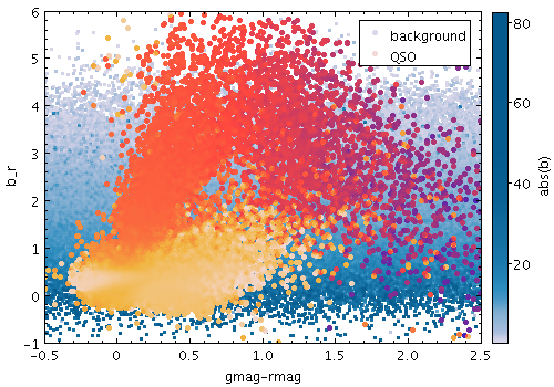
   stilts plot2plane layer1=mark in1=dr5qso.fits
                     x1=psfmag_g-psfmag_r y1=psfmag_u-psfmag_g size1=2
                     shading1=pweighted weight1=z pmap1=sunset
                     layer2=mark in2=:skysim:1_000_000
                     x2=gmag-rmag y2=b_r
                     shading2=weighted weight2=abs(b) auxmap=pubu auxfunc=histogram
                     leglabel1=QSO leglabel2=background legpos=.97,.97 seq=2,1
                     xmin=-0.5 xmax=2.5 ymin=-1 ymax=6

Associated parameters are as follows:

colorN = <rrggbb>|red|blue|...       (Color)

The color of plotted data, given by name or as a hexadecimal RGB value.

The standard plotting colour names are red, blue, green, grey, magenta, cyan, orange, pink, yellow, black, light_grey, white. However, many other common colour names (too many to list here) are also understood. The list currently contains those colour names understood by most web browsers, from AliceBlue to YellowGreen, listed e.g. in the Extended color keywords section of the CSS3 standard.

Alternatively, a six-digit hexadecimal number RRGGBB may be supplied, optionally prefixed by "#" or "0x", giving red, green and blue intensities, e.g. "ff00ff", "#ff00ff" or "0xff00ff" for magenta.

[Default: red]

combineN = sum|count|mean|median|...       (Combiner)

Defines how values contributing to the same pixel are combined together to produce the value assigned to that pixel (and hence its colour).

When a weight is in use, mean or sum are typically sensible choices. If there is no weight (a pure density map) then count is usually better, but in that case it may make more sense (it is more efficient) to use one of the other shading modes instead.

The available options are:

• sum: the sum of all the combined values per bin
• count: the number of non-blank values per bin (weight is ignored)
• mean: the mean of the combined values
• median: the median
• q1: first quartile
• q3: third quartile
• min: the minimum of all the combined values
• max: the maximum of all the combined values
• stdev: the sample standard deviation of the combined values
• stdev_pop: the population standard deviation of the combined values
• hit: 1 if any values present, NaN otherwise (weight is ignored)

[Default: mean]

pclipN = <lo>,<hi>       (Subrange)

Defines a subrange of the colour ramp to be used for Aux shading. The value is specified as a (low,high) comma-separated pair of two numbers between 0 and 1.

If the full range 0,1 is used, the whole range of colours specified by the selected shader will be used. But if for instance a value of 0,0.5 is given, only those colours at the left hand end of the ramp will be seen.

If the null (default) value is chosen, a default clip will be used. This generally covers most or all of the range 0-1 but for colour maps which fade to white, a small proportion of the lower end may be excluded, to ensure that all the colours are visually distinguishable from a white background. This default is usually a good idea if the colour map is being used with something like a scatter plot, where markers are plotted against a white background. However, for something like a density map when the whole plotting area is tiled with colours from the map, it may be better to supply the whole range 0,1 explicitly.

pflipN = true|false       (Boolean)

If true, the colour map on the Aux axis will be reversed.

[Default: false]

pfuncN = log|linear|histogram|histolog|sqrt|square|acos|cos       (Scaling)

Defines the way that values in the Aux range are mapped to the selected colour ramp.

The available options are:

• log: Logarithmic scaling
• linear: Linear scaling
• histogram: Scaling follows data distribution, with linear axis
• histolog: Scaling follows data distribution, with logarithmic axis
• sqrt: Square root scaling
• square: Square scaling
• acos: Arccos Scaling
• cos: Cos Scaling

For all these options, the full range of data values is used, and displayed on the colour bar if applicable (though it can be restricted using the psub option) The Linear, Log, Square and Sqrt options just apply the named function to the full data range. The histogram options on the other hand use a scaling function that corresponds to the actual distribution of the data, so that there are about the same number of points (or pixels, or whatever is being scaled) of each colour. The histogram options are somewhat more expensive, but can be a good choice if you are exploring data whose distribution is unknown or not well-behaved over its min-max range. The Histogram and HistoLog options both assign the colours in the same way, but they display the colour ramp with linear or logarithmic annotation respectively; the HistoLog option also ignores non-positive values.

[Default: linear]

pmapN = <map-name>|<color>-<color>[-<color>...]       (Shader)

Color map used for Aux axis shading.

A mixed bag of colour ramps are available as listed in Section 8.7: inferno, magma, plasma, viridis, cividis, cubehelix, sron, rainbow, rainbow2, rainbow3, pastel, cosmic, ember, gothic, rainforest, voltage, bubblegum, gem, chroma, sunset, neon, tropical, accent, gnuplot, gnuplot2, specxby, set1, paired, hotcold, guppy, iceburn, redshift, pride, rdbu, piyg, brbg, cyan-magenta, red-blue, brg, heat, cold, light, greyscale, colour, standard, bugn, bupu, orrd, pubu, purd, painbow, huecl, infinity, hue, intensity, rgb_red, rgb_green, rgb_blue, hsv_h, hsv_s, hsv_v, yuv_y, yuv_u, yuv_v, scale_hsv_s, scale_hsv_v, scale_yuv_y, mask, blacker, whiter, transparency. Note: many of these, including rainbow-like ones, are frowned upon by the visualisation community.

You can also construct your own custom colour map by giving a sequence of colour names separated by minus sign ("-") characters. In this case the ramp is a linear interpolation between each pair of colours named, using the same syntax as when specifying a colour value. So for instance "yellow-hotpink-#0000ff" would shade from yellow via hot pink to blue.

[Default: inferno]

pquantN = <number>       (Double)

Allows the colour map used for the Aux axis to be quantised. If an integer value N is chosen then the colour map will be viewed as N discrete evenly-spaced levels, so that only N different colours will appear in the plot. This can be used to generate a contour-like effect, and may make it easier to trace the boundaries of regions of interest by eye.

If left blank, the colour map is nominally continuous (though in practice it may be quantised to a medium-sized number like 256).

psubN = <lo>,<hi>       (Subrange)

Defines a normalised adjustment to the data range of the Aux axis. The value may be specified as a comma-separated pair of two numbers, giving the lower and upper bounds of the range of of interest respectively. This sub-range is applied to the data range that would otherwise be used, either automatically calculated or explicitly supplied; zero corresponds to the lower bound and one to the upper.

The default value "0,1" therefore has no effect. The range could be restricted to its lower half with the value 0,0.5.

[Default: 0,1]

weightN = <num-expr>       (String)

Weight coordinate for weighted density shading.

This parameter gives a column name, fixed value, or algebraic expression for the weight coordinate for layer N. The value is a numeric algebraic expression based on column names as described in Section 10.