6 Work and Energy
Work, Energy, and Momentum
When a force acts on a particle, such that its point of action moves through a distance, \(d\), we say that work is done. How much work is done, though? Let’s look at progressively more general examples.
6.1 Constant force parallel to displacement
This is a one dimensional problem. The work done, \(W\), is given by \[ W = F d \] which is the force, \(F\), multiplied by the displacement, \(d\).
Power is the rate of doing work, which we can get by differentiating the work done with respect to time. \[ P = \frac{dW}{dt} = F \frac{d (d)}{dt} = F v \] where \(v\) is the velocity of the particle. (The force, \(F\) is constant so it can be taken outside the derivative).
Note that these expressions also make sense dimensionally.
6.2 Varying force parallel to displacement
If the force varies with position, i.e., force is a function of position \(F(x)\), then we can still calculate the work done by dividing the path into elements of length \(\delta x_i\) over which the force is (almost) constant, \(F(x_i)\), where \(x_i\) is the position of the \(i^\text{th}\) element. The work done by the force moving along each element is then \[ W_i = F(x_i) \delta x_i \] The total work done is then the sum of all the elements \[ W = \sum_i W_i = \sum_i F(x_i) \delta x_i \]
If we take the limit as \(\delta x_i \rightarrow 0\), then we get an integral \[ W = \int_{x=0}^{x=d} F(x) dx \] where \(x=0\) and \(x=d\) are the initial and final positions of the particle.
If we know how \(F(x)\) varies we can calculate the work done.
6.3 Force not parallel to displacement
If the force is not parallel to the displacement, we can still calculate the work done by considering the component of the force parallel to the displacement. If the force makes an angle \(\theta\) with the displacement, then the component of the force parallel to the displacement is \(F \cos \theta\). The work done moving a distance \(d\) is then \[ W = F d \cos \theta\] where \(d\) is the displacement, as shown in Figure 6.1. But this is the definition of the scalar product of \(\vec{F}\) and \(\vec{d}\).
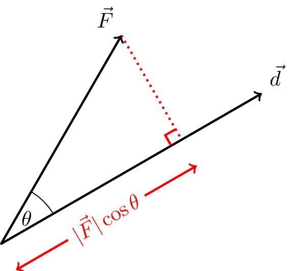
Work done, \(W\), by a force \(\vec{F}\) at an angle \(\theta\) to the displacement \(\vec{d}\) is given by the scalar product of \(\vec{F}\) and \(\vec{d}\), \[ W = \vec{F} \cdot \vec{d} \]
6.4 Example 1: block sliding down a frictionless plane
Consider a block, initially at rest, sliding down a frictionless plane. This is illustrated in Figure 6.2.
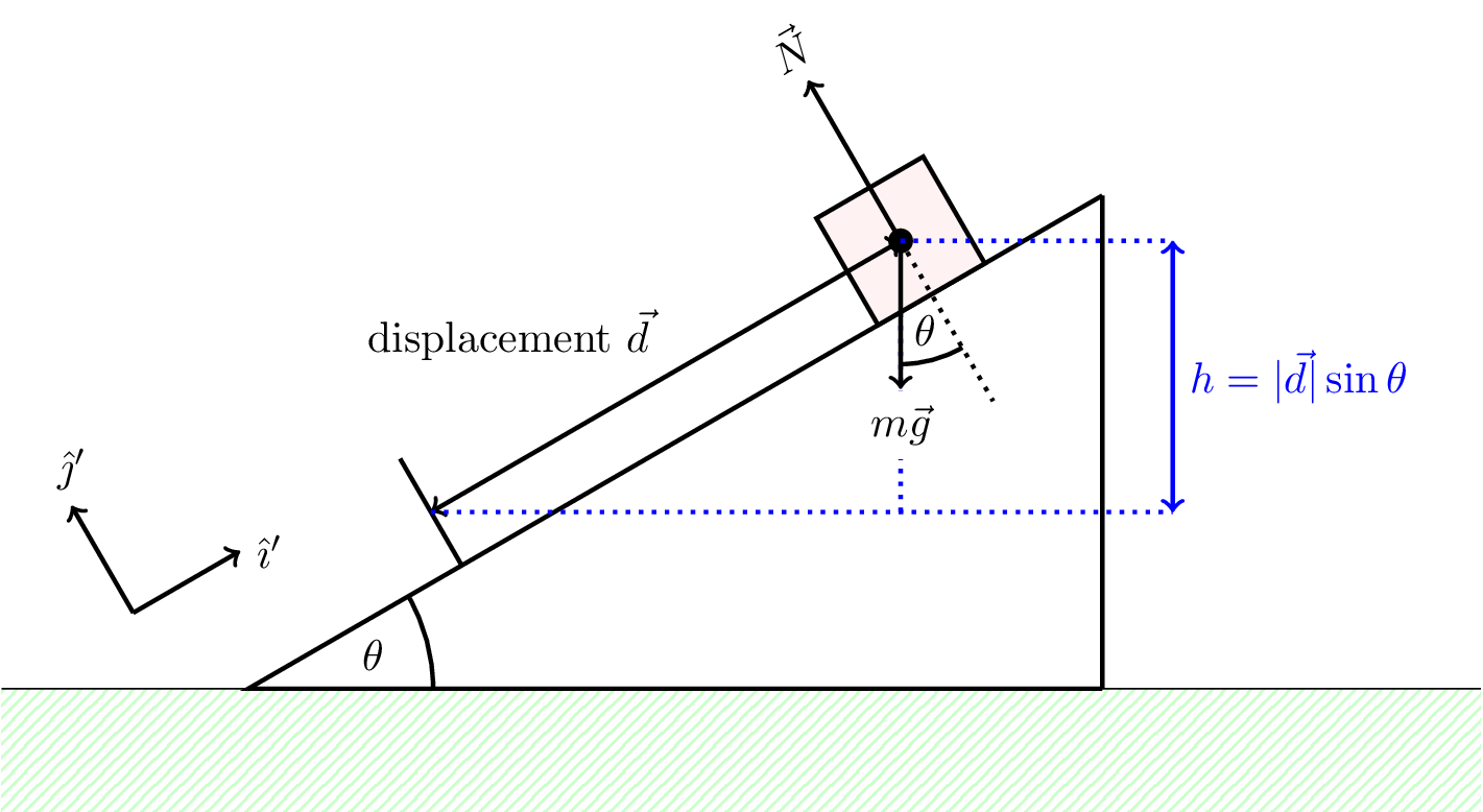
The component of the gravitational force parallel to the plane is \[ mg \sin\theta \] This means that the work done is this component of the force times the distance moved, \(d\), given by \[ W = mgd \sin\theta \] Interestingly, the work done exactly matches the loss of gravitational potential energy, \(mgh\), where \(h = d \sin\theta\) is the vertical distance the block falls through (see Figure 6.2). This is not a coincidence, as we will see later.
6.5 Example 2: circular motion
Consider a particle moving in a circle orbit, as shown in Figure 6.3. The centripetal force is always perpendicular to the motion. The instantaneous displacement, \(d\vec{s}\), is parallel to \(\vec{v}\) because \(\vec{v} = d\vec{s}/dt\).
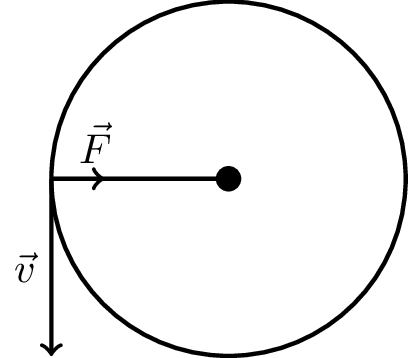
This means that \(\vec{F} \cdot \vec{ds} = 0\) so no work is done.
6.6 Kinetic energy
Consider a force moving through a displacement \(d\), in one dimension. The work done, \(W\) is given by \[ \Delta W = \int_0^d F(x) dx \] The force gives rise to an acceleration, which results in a change of velocity (or speed in one dimension).
If we assume the initial velocity \(= 0\), and the final velocity \(= v_f\), we can compare this with the work done as follows.
\[ \Delta W = \int_0^d ma(x) dx \] \[ \Delta W = \int_0^d mv \frac{dv}{dx} dx = \int_0^{v_f} mv dv \] where we have used the cain rule to write \(\frac{dv}{dt} = \frac{dv}{dx} \frac{dx}{dt} = v \frac{dv}{dx}\). \[ \Delta W = \left[ \frac{mv^2}{2} \right]^{v_f}_0 = \frac{1}{2} m v_f^2 \] which is the kinetic energy associated with the motion of the particle.
Therefore, work done produced kinetic energy.
If the initial velocity \(= v_0\), we would obtain
Work done \(\Delta W\) = change in kinetic energy \[ \Delta W = \frac{1}{2} m v_f^2 - \frac{1}{2} m v_i^2 \] where \(v_i\) is the initial velocity, and \(v_f\) is the final velocity.
6.6.1 Example: kinetic friction
Consider a block sliding along a rough surface that is brought to rest from a speed \(v_i\) by a kinetic friction force of magnitude \(\mu_k N\), where \(N\) is the magnitude of the normal reaction force. This is shown in Figure 6.4.
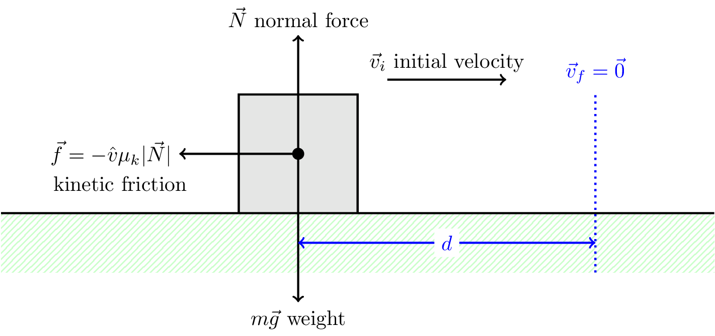
\[ \Delta W = 0 - \frac{1}{2} m v_i^2 \] \[ F = \mu_k N = \mu_k mg \] \[ \Delta W = \vec{F} \cdot \vec{d} = -F d = -\mu_k mgd \] \(\Delta W < 0\) as particle loses kinetic energy. We can equate \(\Delta W\) with the kinetic energy to get \[ \frac{1}{2} m v_i^2 = \mu_k mgd \] \[ \therefore v_i^2 = 2 \mu_k gd \]
6.6.2 KE in different reference frames
Note that the kinetic energy is not the same in different reference frames, just as the velocity is not the same in different reference frames. This means that statements regarding conservation of energy must be restricted to a single reference frame.
6.7 Potential energy
If a force is a function of position (or a constant) we can define a potential difference, \(\Delta V\), of a particle, as the work done against the force in moving from one position, \(A\), to another position, \(B\). This is given, in one dimension, by \[ \Delta V = V(B) - V(A) \] where \[ V(A) = - \int_0^A F(x) dx \tag{6.1}\] where the negative sign is because the force is acting against the force. The integration is from zero here, but it could be some other reference point, e.g., \(-\infty\), where the potential \(V\) is defined to be zero. \[ V(B) = - \int_0^B F(x) dx \]
Examples of forces that depend only on a particle’s position include gravity and the electrostatic force.
\(V(A)\) is a scalar function of position, known as the potential.
From Equation 6.1, we can see that a differential from will also hold, \[ F(x) = - \frac{dV(x)}{dx} \] which is a direct consequence of the definition of the potential.
The force \(F(x)\) is minus the gradient of the potential \(V(x)\), \[ F(x) = - \frac{dV(x)}{dx} \]
The zero of the potential is not fixed and depends on the (sometimes arbitrary) choice of reference point. Adding a constant to the potential does not change the gradient or, therefore, the force. The derivative of a constant is zero.
We can therefore choose a convenient zero point for the potential, appropriate to the problem being studies.
6.7.1 Example 1: lifting a particle against gravity
Consider lifting a particle through a height \(h\), doing work against gravity, as shown in Figure 6.5.
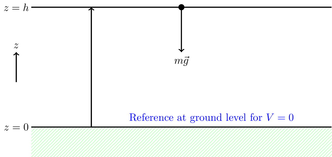
The potential difference is given by \[ \Delta V = V(h) - V(0) \] \[ \Delta V = - \int_0^h (-mg) dz = mgh \] Note the minus sign because we’ve defined positive \(z\) to be up. \[ \therefore V(h) = mgh + V(0) \] where \(V(0)\) is the potential at \(z=0\) which we can choose to be our reference level with a potential of zero.
6.7.2 Example 2: particle escaping gravity
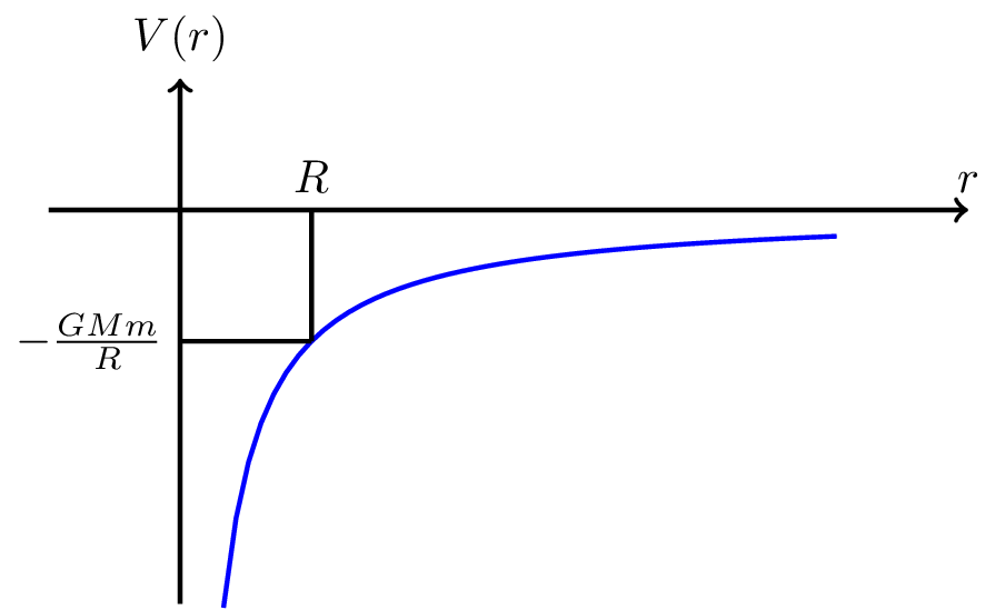
Consider a particle escaping form the surface of a planet, as illustrated by Figure 6.6.
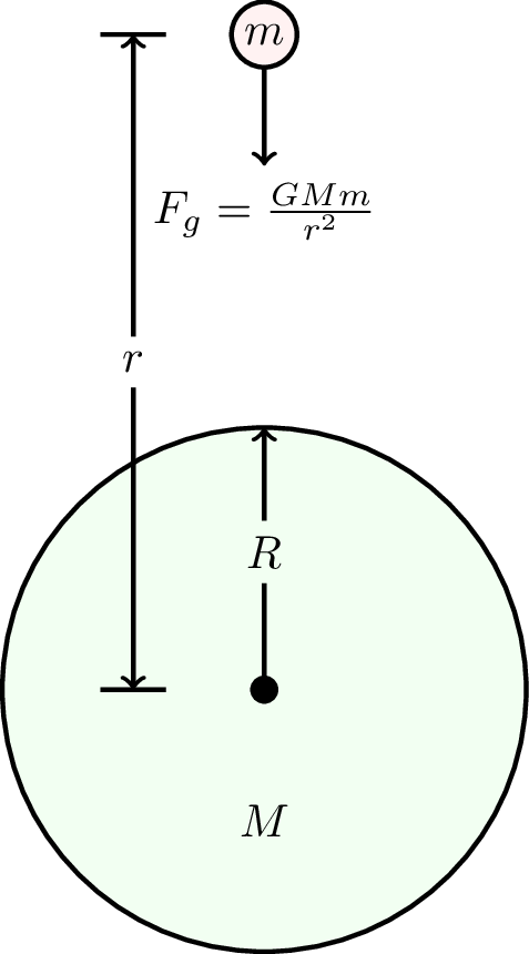
Newton’s law of gravity states that the force between the particle of mass \(m\) and the planet of mass \(M\) is given by \[ F = - \frac{GMm}{r^2} \] where \(r\) is the distance between the particle and the centre of the planet, and \(G\) is the gravitational constant. To escape gravity we need to take the particle from the surface at radius \(R\) to \(\infty\). The work done against the force of gravity will be \[ \Delta V = V(\infty) - V(R) \] \[ \Delta V = \int_R^\infty \left(-\frac{GMm}{r^2}\right) dr = GMm \left[ -\frac{1}{r} \right]_R^\infty \] \[ \therefore \Delta V = \frac{GMm}{R} \] for escape to infinity, i.e., the particle needs to gain this energy.
6.7.3 Example 3: horizontal stretched spring
We can caluclate the work done by moving the block and stretching the spring from \(0\) to \(x\), as show in Figure 6.7.
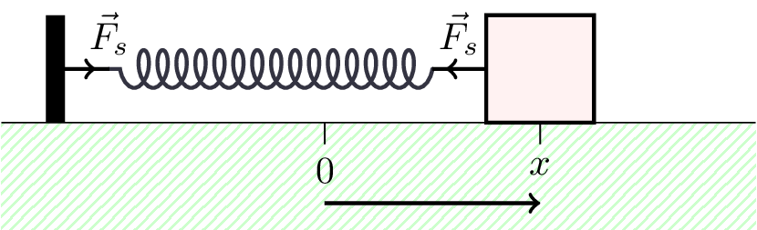
\[ \Delta V = V(x) - V(0) \] \[ \Delta V = - \int_0^x (-kx') dx' = \frac{1}{2} kx^2 \] where \(k\) is the spring constant. \[ \therefore V(x) = \frac{1}{2} kx^2 + V(0) \] Normally choose \(V(0) = 0\), i.e., origin at equilibrium position.
6.8 Conservation of energy
The mechanical energy we’ve looked at so far can be divided into two parts: kinetic energy due to the motion, and potential energy due to the position. The total mechanical energy is the sum of the kinetic and potential energies,
When work is done by, e.g., friction or drag, energy is lost mainly as heat, sound, etc.
The total energy of a closed system is constant in time. Energy can be converted from one form to another, but not created or destroyed.
By a closed system we mean one that is not acted on by external forces. This is a very important point. If external forces are acting on the system, then the total energy of the system is not conserved.
If there is an external force, the total force acting on the particle is written as \[ F_\text{ext} + F(x) = ma \] Therefore the work done by the external force can be written as \[ \Delta W_\text{ext} = \int_{x_0}^{x_1} F_\text{ext} dx = \int_{x_0}^{x_1} ma dx - \int_{x_0}^{x_1} F(x) dx \] From before we have that \[ \int_{x_0}^{x_1} ma dx = \int_{x_0}^{x_1} mv \frac{dv}{dx} dx = \frac{1}{2} m (v_1^2 - v_0^2) = \Delta K \] and \[ - \int_{x_0}^{x_1} F(x) dx = V(x_1) - V(x_0) = \Delta V \] so \[ \Delta W_\text{ext} = \Delta K + \Delta V \] where \(\Delta K\) is the change in kinetic energy, and \(\Delta V\) is the change in potential energy. I.e., external force leads to changes in both KE and PE.
Equally, if external force is zero, total change in KE and PE is zero, \[ 0 = \Delta K + \Delta V \] This is conservation of energy.
6.8.1 Example: escape velocity
Consider a particle with just enough kinetic energy to escape to infinity from the surface of a planet (ignoring resistance from the atmosphere of the planet). The initial configuration is shown in Figure 6.8.
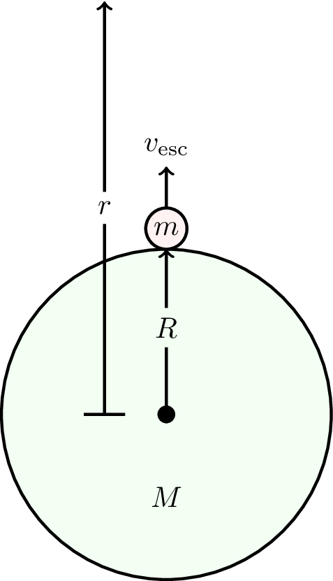
If the particle just escapes to infinity, this means that the velocity \(v \to 0\) as \(r \to \infty\). The final total energy is zero, if we define the zero point of the gravitational potential to be at infinity (see Figure 6.9). We can then use conservation of energy \[ \underbrace{0}_{\color{blue}\text{final energy}} = \underbrace{-\frac{GMm}{R}}_{\color{blue}\text{initial PE}} + \underbrace{\frac{1}{2}mv^2_\text{esc}}_{\color{blue}\text{initial KE}} \]
\[ \therefore v_\text{esc} = \sqrt{\frac{2GM}{R}} = 11.2 \text{ km s}^{-1} \text{ for Earth.} \]
What would happen if the planet was shrunk so that \(R = GM/c^2\)?
6.8.2 Proof of conservation of energy
This isn’t examinable but is included for those interested in seeing the proof.
Let the total energy of a mechanical system be \[ E_\text{tot} = \frac{1}{2} mv^2 + V(x) \] The total energy, \(E_\text{tot}\) depends on arbitrary choices of the inertial frame which affects KE and the choice of the zero point of the potential \(V(0)\) which affects PE.
If \(E_\text{tot}\) is conserved, it means that it is not changing with time, i.e., \[ \frac{dE_\text{tot}}{dt} = 0 \] This means \[ \frac{dE_\text{tot}}{dt} = \frac{d}{dt} \left( \frac{1}{2} mv^2 + V(x) \right) = 0 \] Applying the chain rule to both terms, \[ \frac{dR_\text{tot}}{dt} = \frac{1}{2} m 2v \frac{dv}{dt} + \frac{dV(x)}{dx} \frac{dx}{dt} \] \[ = mva + v \times \underbrace{\frac{dV(x)}{dx}}_{\color{blue}\text{gradient of potential} = -F} \] \[ \therefore \frac{dE_\text{tot}}{dt} = v \left( ma - F \right) = 0\] by Newton’s second law.
So, in the absence of external forces, energy is conserved.
Notes
- Newton’s first law: total energy depends on reference frame, but energy is conserved in all reference frames, if it is conserved in one.
- Newton’s third law: must include both forces in an action-reaction pair, to avoid external forces
- In practice, for gravity problems including the Earth, the work done on the Earth is \(\simeq 0\) because displacement is tiny
- Energy conservation often provides an alternative approach to Newton’s laws for solving mechanics problems (and can often be easier!)
6.9 Conservative forces
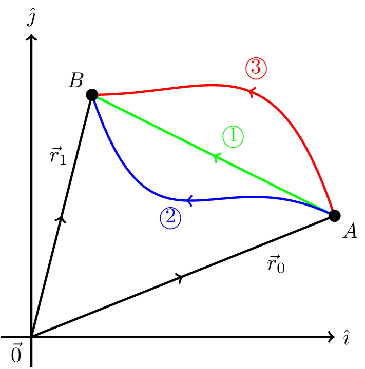
Conservative forces can be written as minus the gradient of a potential. Consider the work done against a force \(\vec{F}(\vec{r})\). We can only define a potential when \[ \underbrace{V(\vec{r}_1) - V(\vec{r}_0)}_{\text{\color{blue} depends only on end points}} = \underbrace{\int_{\vec{r}_0}^{\vec{r}_1} \vec{F}(\vec{r}) \cdot d\vec{r}}_{\text{\color{blue}must be independent of path}} \]
Forces \(\vec{F}(\vec{r})\) for which a potential \(V(\vec{r})\) can be defined are called conservative forces. The work done by a conservative force around a closed loop is zero.
In 1D \[ F = - \frac{dV}{dx} \] In 3D \[ \vec{F}(\vec{r}) = - \text{gradient} (V(\vec{r})) = -\vec{\nabla} V(\vec{r}) \] where the gradient is defined in the following way \[ \vec{F}(\vec{r}) = -\vec{\nabla} V(\vec{r}) = -\frac{\partial V}{\partial x} \hat{\imath} - \frac{\partial V}{\partial y} \hat{\jmath} - \frac{\partial V}{\partial z} \hat{k} \] Gravity and electrostatic forces are examples of conservative forces.
Don’t worry about the 3D maths and the path integral described above; that will be covered in maths units later. The important physics point is that for a conservative force the potential difference between two points \(A\) and \(B\) only depends on those points, it does not matter what path the particle took to get from \(A\) to \(B\).
6.10 Collisions with conservation of energy and momentum
We are going to consider collisions between particles in one frame of reference so we can consider energy to be conserved, as well as momentum, as we will be considering a closed system (i.e., no external forces). We’ll start by considering a one-dimensional example.
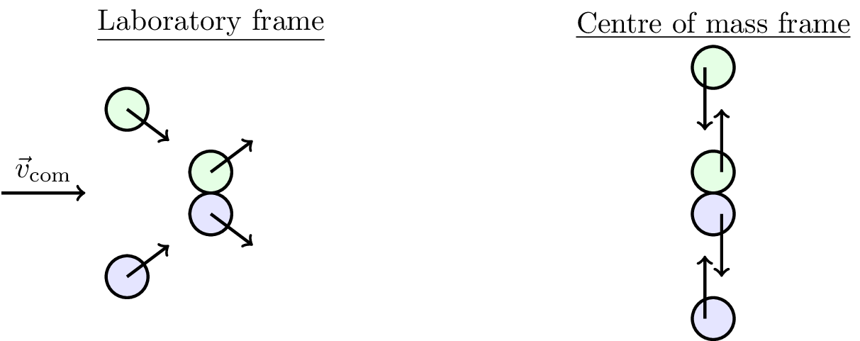
Note that sometimes we can reduce a 2D problem to a 1D problem by working in the centre of mass frame, which can make things simpler. See, e.g., Figure 6.11. This works fine for point particles.
6.10.1 Collision in 1D
Consider two particles colliding in 1D as shown in Figure 6.12.
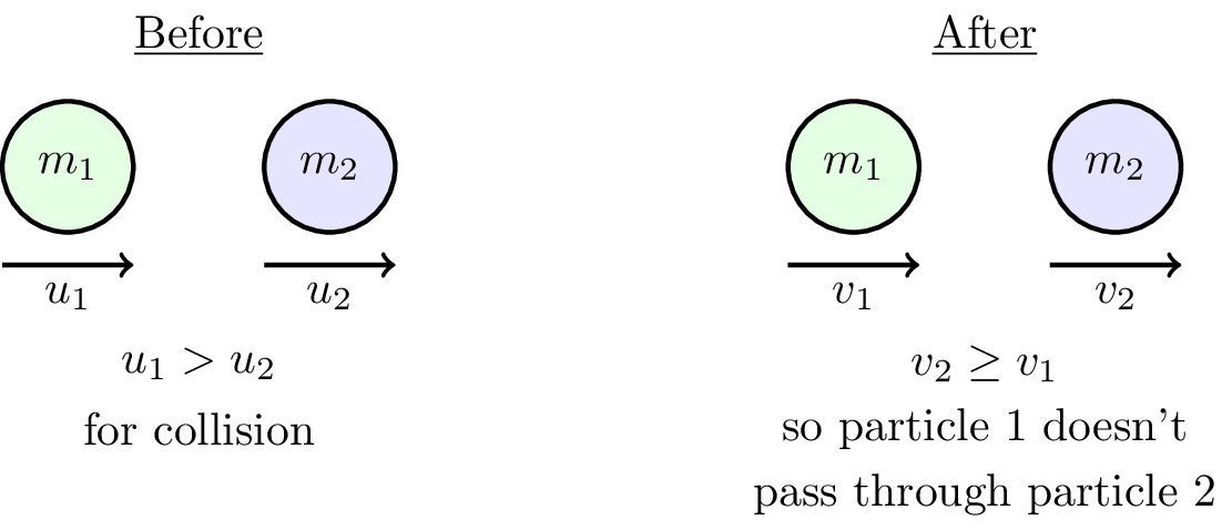
Before the collision \(u_1 > u_2\) otherwise the particles would not collide. After the collision \(v_2 \ge v_1\) because the particles can’t pass through each other (at leats in classical mechanics).
Conservation of momentum gives us \[ m_1 u_1 + m_2 u_2 = m_1 v_1 + m_2 v_2 \]
Note, however, that not all collisions conserve kinetic energy (in general some energy will be lost to heat, sound, etc.). We can quantify this by defining a coefficient of restitution.
The coefficient of restitution, \(e\), is defined as the ratio of the relative velocity of separation to the relative velocity of approach, \[ e = \frac{\text{relative speed after collision}}{\text{relative speed before collision}} \] \[ e = \frac{| v_2 - v_1 |}{| u_1 - u_2 |} \] \[ 0 \le e \le 1 \] These relative speeds are along the line of impact (best suited to 1D problems). There are two special cases
- \(e = 1\) for a perfectly elastic collision
- \(e = 0\) for a perfectly inelastic collision
Perfectly elastic collisions: If \(e = 1\) we have perfectly elastic collisions, so \(u_1 - u_2 = v_2 - v_1\), or \(u_1 + v_1 = u_2 + v_2\). Conservation of momentum can be written at \[ m_1 (u_1 - v_1) = m_2 (v_2 - u_2) \] Multiplying these two expressions together (and then multiplying by \(1/2\)) gives \[ \frac{1}{2} m_1 u_1^2 + \frac{1}{2} m_2 u_2^2 = \frac{1}{2} m_1 v_1^2 + \frac{1}{2} m_2 v_2^2 \] i.e., perfectly elastic collisions result in conservation of energy.
Perfectly inelastic collisions: If \(e = 0\) we have perfectly inelastic collisions, \(v_2 = v_1 = v\), so the particles stick together. \(v\) will be equal to \(v_\text{com}\), the velocity of the centre of mass.
If \(v = 0\) the final KE \(=0\) which happens if \(m_1 u_1 = -m_2 u_2\), i.e., if \(v_\text{com} = 0\) before the collision because momentum is still conserved.
If we are in the centre of mass frame then the total momentum is zero, both before and after the collision. Hence, in 1D (for simplicity) we have \[ m_1 u_1 + m_2 u_2 = 0 \] and \[ m_1 v_1 + m_2 v_2 = 0 \] The equation for the coefficient of restitution, also in 1D, is then \[ e = \frac{| v_2 - v_1 |}{| u_2 - u_1 |} = \frac{v_2 - v_1}{u_1 - u_2} \] These can be combined, with some algebra, to give \[ \frac{\text{Total final KE}}{\text{Total initial KE}} = e^2 \] But this is only true in general in the centre of mass frame.
6.10.2 General momentum conservation
We can generalise our analysis beyond the one dimensional case, as shown in Figure 6.13. If we use vectors, each component of the momentum \(\vec{p}\) is separately conserved.
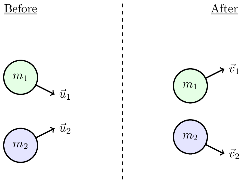
We can write the conservation of momentum as \[ \vec{p}_\text{before} = \vec{p}_\text{after} \]
This gives \[ m_1 \vec{u}_1 + m_2 \vec{u}_2 = m_1 \vec{v_1} + m_2 \vec{v_2} \] which can be expanded to give three equations for conservation of energy in the \(x\), \(y\), and \(z\) directions. I.e., \[ m_1 u_{1x} + m_2 u_{2x} = m_1 v_{1x} + m_2 v_{2x} \] \[ m_1 u_{1y} + m_2 u_{2y} = m_1 v_{1y} + m_2 v_{2y} \] \[ m_1 u_{1z} + m_2 u_{2z} = m_1 v_{1z} + m_2 v_{2z} \] where \(u_{1x}\) is the \(x\) component of the velocity of particle 1 before the collision, etc. and momentum is separately conserved in each direction.
Also, if the collision is perfectly elastic, kinetic energy is conserved so \[ \frac{1}{2} m_1 u_1^2 + \frac{1}{2} m_2 u_2^2 = \frac{1}{2} m_1 v_1^2 + \frac{1}{2} m_2 v_2^2 \] If you can reduce the problem to 1D, e.g., for two particles in the centre of mass frame, then the coefficient of restitution can be used.