2 Motion in 1D
Displacement, Velocity, Acceleration
2.1 Units, dimensions, estimation
Before we start to think about mechanics it will be really useful to discuss units, dimensions, and estimation. This is important because all of the physics equations you write down must be dimensionally correct otherwise they won’t make sense (e.g., “how long is piece of string?”, answer “15 seconds” is not sensible). Estimation will also be extremely useful for checking your answers (e.g., “how long will it take to warm up my soup?”, answer “\(5 \times 10^{17}\) seconds” is not sensible; a universe with intelligent life can be created in less time).
2.1.1 Dimensional analysis
Each term in an equation has to have the same “dimensions”, i.e., units, for the equation to make sense. Units can be combined by multiplication and division. Area, \(A\) for example, is given by multiplying two lengths together so has dimensions of length squared. We use square brackets to denote “dimension of”, so this is written \([A] = L^2\) to show that area has has the dimensions of length squared. The units of some common quantities are given in Table 2.1. You can add to this list as you encounter new quantities and units.
| Quantity | Dimension |
|---|---|
| Length | \(L\) |
| Mass (\(M\)) | \(M\) |
| Time | \(T\) |
| Area (\(A\)) | \(L^2\) |
| Volume (\(V\)) | \(L^3\) |
| Speed | \(L/T\) |
| Acceleration | \(L/T^2\) |
| Force (\(F\)) | \(ML/T^2\) |
| Pressure (\(F/A\)) | \(M/LT^2\) |
| Density (\(M/V\)) | \(M/L^3\) |
| Energy | \(ML^2T^{-2}\) |
| Power | \(ML^2T^{-3}\) |
The superpower you gain with dimensional analysis is the ability to generate plausible equations. But with great power comes great responsibility; the equations you generate this way don’t have to be correct but they often provide useful insight. Let’s look at an example.
A mass on the end of a string is moving in a circle at constant speed. What is the force exerted on the mass by the string?
What might the answer depend on? Maybe the mass \(m\), speed \(v\), radius \(r\) of the circle. These have dimensions \[ [m] = M \] \[ [v] = L/T \] \[ [r] = L \] and the dimension of the force, \(F\), is \[ [F] = ML/T^2 \] So we need to combine \(m\), \(v\), and \(r\) to get something that has the same dimensions as \(F\). We find that the following combination works \[ F \propto \frac{mv^2}{r}. \] We’ve used “proportional to”, \(\propto\), because we can always multiply by a constant that has no dimensions. In this case, the constant is \(1\), and we know this is the right answer!
2.1.2 Significant figures
A friend asks you, “How old is the universe?” Conveniently, another friend, who is an astronomer, had just told you that the Universe is 14 billion years old. So you answer, “The universe is 14 billion years and 2 hours old.”
In physics it is important to use an appropriate number of significant figures to give some idea of the precision of a measurement. A reliably known digit is called a significant figure. So, e.g., if we measure the height of a person to be 1.7 m, we are saying that we know the length to within 0.1 m. If we measure the length of a table to be 1.75 m, we are saying that we know the length to within 0.01 m. The number of significant figures is the number of digits that are known with certainty plus one estimated digit. So, e.g., if we measure the length of a table to be 1.753 m, we are saying that we know the length to within 0.001 m.
- Significant figures are “reliable digits” plus one “estimated digit”.
- When multiplying or dividing quantities, the result should have the same number of significant figures as the quantity with the fewest significant figures.
- When adding or subtracting quantities, the result should have the same number of decimal places as the quantity with the fewest decimal places.
2.1.3 Estimation
Estimation works by using “orders of magnitude”. For example, the height of a person is \(\sim 10^0 = 1 \text{ m}\). Even though the average height of a person is closer to 2 m and there are variations between people, this doesn’t matter if we’re interested in making an order of magnitude estimate. Why might this be helpful? It immediately tells us that if, e.g., we want to build a new lecture theatre we should be thinking about rooms that are \(\sim 10^0 \text{ m}\) high (perhaps in the range 0.1–100 m), and certainly not \(\sim 10^{-8} \text{ m}\) or \(\sim 10^{10} \text{ m}\). Similarly, if we performed some calculation to estimate the height of a person and the answer wasn’t \(\sim 10^0 \text{ m}\) we would know that we had made a mistake.
The power of these “order of magnitude” estimates is that we don’t need particularly precise data. In the example above we only needed to know that the height of a person is roughly \(10^0\text{ m}\), and any reasonable guess would be good enough to rule out building an absurdly small or large building. Of course, being more precise would require more work.
How many grains of sand are there on a patch of beach 500 m long and 100 m wide?
This sounds impossible to answer, and it is practically impossible if you want to know precisely the number of grains. However, an estimate is quite feasible.
We need to guess the size of a grain of sand, and the depth of the sand on a beach. Let’s say a grain of sand has a diameter of 1 mm, and the depth of sand is 2 m.
The volume of sand on the beach is approximately \[ V_\text{b} \simeq 500 \times 100 \times 2 = 10^5 \text{ m}^3. \]
The volume of a spherical grain of sand is approximately \[ V_\text{s} \simeq \frac{4}{3} \pi \left( \frac{1.0 \times 10^{-3}}{2} \right)^3 \simeq 10^{-9} \text{ m}^3 \] (you can approximate \(\pi\) as 3 to do these calculations in your head).
The number of grains is then \[ N \simeq \frac{V_\text{b}}{V_\text{s}} \simeq 10^{14}. \] where we have neglected the packing efficiency of grains (there is some space between grains), and assumed the grains fill up most of the volume.
Note that this estimate doesn’t change much if, e.g., the depth is 1 m or 3 m, or if the diameter of a grain of sand is 1.5 mm or 2 mm, as long as we have a reasonable, order of magnitude estimate.
Remember that you can use dimensional analysis and estimation throughout the course.
2.1.4 Some examples
It is always good to consolidate your physics knowledge by trying some example questions.
The drag force on a sphere falling through the air depends on the air density, \(\rho\), the radius of the sphere, \(r\), and the speed of the sphere, \(v\). Use dimensional analysis to come up with an equation for the drag force.
2.2 Displacement, velocity, and acceleration
OK, on to mechanics!
We are interested in determining the equations of motion of physical systems that describe how they evolve as a function of time. For example, how far a train has moved along a track, how fast is it moving, what is its acceleration? To do this we will need to know something about vectors and calculus. These concepts will become increasingly useful throughout your physics degree.
Let’s start by looking at motion in one dimension to familiarise ourselves with the basics of displacement, velocity, and acceleration. We’ll then generalise things to two and three dimensions, making use of vectors. (And ultimately to four dimensions, but that’s a story for another time).
2.2.1 Displacement
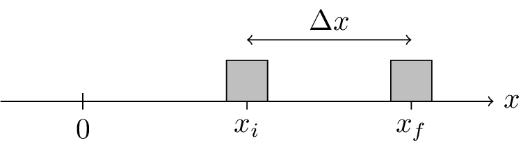
Consider a train moving along a track. At some initial time \(t_\text{i}\) the train is a distance \(x_\text{i}\) along the track. At some later time \(t_\text{f}\) the train has moved further along the track to a position \(x_\text{f}\). The displacement of the train is the difference between the final and initial positions, \[ \Delta x = x_\text{f} - x_\text{i}. \] The Greek capital letter \(\Delta\), “delta”, is often used to denote a large change such as this. (A lower case delta is often used to represent small changes, \(\delta \ll 1\)).)
2.2.2 Average velocity
The velocity is the rate at which position changes. The average velocity, \(v_\text{av}\) is given by the change in position divided by the change in time, \[ v_\text{av} = \frac{\Delta x}{\Delta t}. \] where \(\Delta t = t_\text{f} - t_\text{i}\) is the change in time.
This means that the \[ \text{average velocity} = \frac{\text{total displacement}}{\text{total time}}. \] which is the gradient of a straight line from \((x_\text{i}, t_\text{i})\) to \((x_\text{f}, t_\text{f})\).
It has been speculated that the Oumuamua comet that passed through the solar system in 2017 was an alien spacecraft. It was observed leaving the solar system, moving along an approximately straight line. On \(7^\text{th}\) October it was observed to be \(1.47 \times 10^{11} \text{ m}\) from the Sun and on \(28^\text{th}\) October is was observed to be \(2.29 \times 10^{11} \text{ m}\) from the Sun. What was its average velocity?
The average velocity is given by \[ v_\text{av} = \frac{\Delta x}{\Delta t} \] In this case \(\Delta x = (2.29 - 1.47) \times 10^{11} = 8.2 \times 10^{10} \text{ m}\) and \(\Delta t = 21 \text{ days} = 1.8 \times 10^6 \text{ s}\). So the average velocity is \[ v_\text{av} = \frac{8.2 \times 10^{10}}{1.8 \times 10^6} \text{ m/s} = 4.6 \times 10^4 \text{ m/s} = 46 \text{ km s}^{-1} \]
This is larger than the escape velocity of the solar system at this distance (\(\simeq 17 \text{ km s}^{-1}\)). When we discuss energy later in the course you’ll be able to figure this out yourselves.
2.2.3 Relative velocity
When we are talking about velocity, we are considering a specific frame of reference that our coordinate system is attached to.
A frame of reference is an extended object whose parts are at rest relative to each other.
The velocity will be different in different frames of reference. For example, consider walking along the aisle of a train. If you are walking towards the front of a train at \(v_\text{t} = 1 \text{ m s}^{-1}\), and the train is moving at \(v_\text{tp} = 10 \text{ m s}^{-1}\) relative to the platform, then you are moving at \(v_\text{p} = 11 \text{ m s}^{-1}\) relative to the platform. This is called the relative velocity. \[ v_\text{p} = v_\text{t} + v_\text{tp}. \]
This equation is not true in general and only applies for small velocities \(v \ll c\), where \(c\) is the speed of light. For velocities that are a significant fraction of the speed of light we have to consider special relativity. You will study this next year, or you can look it up in the course textbook.
2.2.4 Instantaneous velocity
In general, the velocity can change over time. For example, the train might be speeding up or slowing down.
How can we define the velocity at an instant in time? We can look at the average velocity over progressively smaller intervals of time. This is shown in Figure 2.2, where we are considering the velocity at some time \(t_0\) and position \(x_0\), denoted by the point \(P\) in the figure. As we estimate the velocity using shorter and shorter time intervals, our velocity estimate gets closer and closer to the tangent at point \(P\).
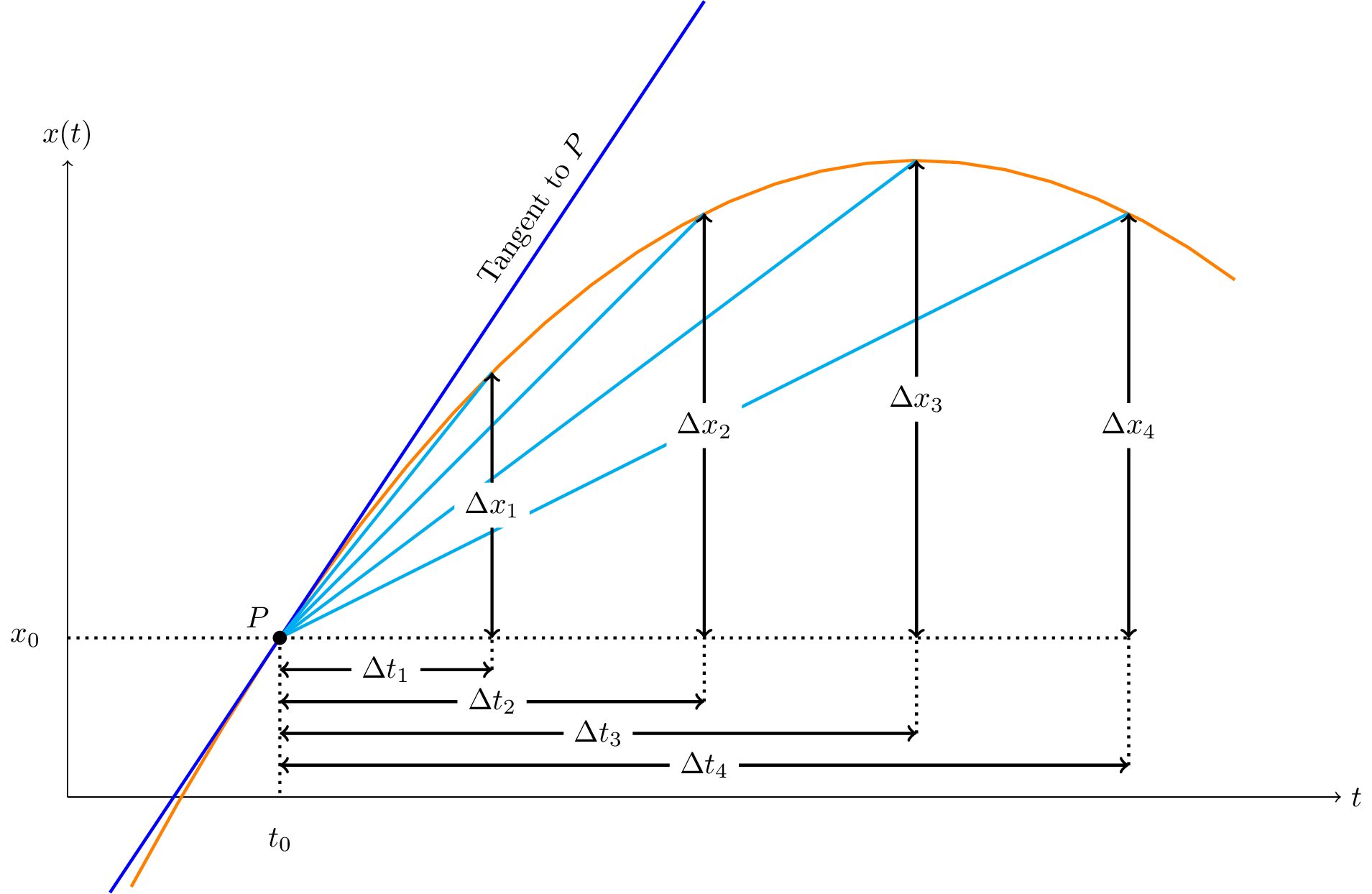
We write this mathematically at a limit, \[ v(t_0) = \lim_{\Delta t \to 0} \frac{\Delta x}{\Delta t} \] which is the slope of the curve at point \(t_0\). This is the derivative of position \(x\) with respect to time \(t\), and speed is the rate of change of position. \[v = \frac{dx}{dt}\] This is often written as \(v = \dot{x}\), and we say “\(x\) dot”.
The derivative of a function \(f(t)\) with respect to \(t\) is defined as \[ \frac{df(t)}{dt} = \lim_{h \to 0} \frac{f(t+h) - f(t)}{h}. \] You can try this with, e.g., \(f(t) = t^2\).
Galileo drops a ball from the top of the leaning tower of Pisa. The position of the ball is described approximately as \(s(t) = 5t^2 \text{ m}\) where the time, \(t\), is measured in seconds after the ball is released, and the vertical position, \(x\), is measured downwards in metres. What is the velocity at any time \(t\)?
The velocity is the derivative of position with respect to time, \[ v = \frac{ds}{dt} = 10t \text{ m s}^{-1}. \]
2.2.5 Acceleration
Similarly, the acceleration, \(a\), is given by the rate of change of velocity with time, \[ a = \frac{dv}{dt} = \frac{d^2 x}{dt^2} \] which can also be written \[ a = \ddot{x} \] and we say “\(x\) double dot”.
It is clear that some knowledge of calculus is going ot be useful for solving mechanics problems. In fact, calculus is going to be really important throughout your physics degree. It is therefore highly recommended that you practice differentiating some standard functions so that you can concentrate on the underlying physics rather than the mathematics.
Here are some examples of functions that you should be able to differentiate by the end of the course. You will have more practice of this elsewhere in your degree programme.
- Polynomial functions such as \(y(x) = ax^n + bx^m\).
- Trigonometric functions such as \(y(x) = \sin(x)\).
- Natural logarithms such as \(y(x) = \ln(x)\).
- Product rule for \(y(x) = f(x) g(x)\).
- \(y(x) = x^2 \sin(x)\).
- Chain rule for \(y(x) = f(g(x))\).
- \(y(x) = \sin(x^2)\).
2.2.6 Integration
So far we have used differentiation to get the “rate of change” of certain quantities. Velocity is the rate of change of position; acceleration is the rate of change of velocity. How do we go the other way?
We use integration, which is the opposite of differentiation. The fundamental theorem of calculus which states that \[ f(x) = \int_0^x \frac{df}{dx} dx. \]
For example, if we have a graph of velocity versus time and we want to know the change in displacement we can integrate.
\[ \int_{x_0}^{x_1} dx = \int_{t_0}^{t_1} v dt \] which is the area under the curve between times \(t_0\) and \(t_1\). This gives us \[ \Delta x = x_1 - x_0 = \int_{t_0}^{t_1} v dt \]
It is easy to see why this is the case for constant velocity. However, if you imagine dividing the timeline into segments where the velocity is approximately constant you visualise how the general result holds.
Here are some examples of functions that you should be able to integrate by the end of the course. You will have more practice of this elsewhere in your degree programme.
- Polynomial functions such as \(y(x) = ax^n + bx^m\).
- Trigonometric functions such as \(y(x) = \sin(x)\).
- Integration to obtain natural logarithms such as \(y(x) = 1/x\).
- Integration by parts.
- Integration by substitution.
2.2.7 Constant acceleration
It is very useful to consider a system in which there is constant acceleration, \(a\). We can write this acceleration in the following way. \[ \frac{d^2 x}{dt^2} = \frac{dv}{dt} = a \] We can integrate this equation, \[ \int_{v_0}^{v_1} dv = \int_{t_0}^{t_1} a dt \] \[ v_1 - v_0 = a(t_1 - t_0) \] We can start measuring time from \(t_0 = 0\) to get \[ v_1(t_1) = v_0 + a t_1 \] where \(t_1\) is the elapsed time. Note that \(v_1\) is a function of \(t_1\) because it depends on \(t_1\). Different elapsed times result in different velocities.
Integrating once more, again assuming we start timing at \(t_0 = 0\), we get \[ x_1 - x_0 = \int_{0}^{t_1} v(t) dt \] \[ x_1 - x_0 = \int_{0}^{t_1} (v_0 + a t) dt \] If we measure displacement from \(x_0 = 0\) we get \[ x_1(t) = v_0 t_1 + \frac{1}{2} a t_1^2 \]
Finally, we can derive one more equation using an integration “trick”. Note that we can write \[ \frac{d^2 x}{dt^2} = \frac{dv}{dt} = \frac{dv}{dx} \frac{dx}{dt} = v \frac{dv}{dx} \] where we have used the chain rule, considering \(v\) to be a function of distance, \(v(x)\). We can then write constant acceleration as \[ v \frac{dv}{dx} = a \] and rearrange to get \[ \int_{v_0}^{v_1} v dv = \int_{s_0}^{s_1} a dx \] \[ \frac{v_1^2}{2} - \frac{v_0^2}{2} = a (s_1 - s_0) \] Again assuming \(s_0 = 0\) we get \[ v_1^2 = v_0^2 + 2 a s_1 \]
These are the equations of motion for constant acceleration. They are more often written as follows.
2.2.8 SUVAT equations
You will often hear reference to the “SUVAT” equations. These are the set of equations derived above that describe motion with constant acceleration. This term is frequently used in the UK A-Level education system, but you might not hear it elsewhere. The equations are:
- \(s\) is displacement
- \(u\) is the initial velocity
- \(v\) is the final velocity
- \(a\) is the constant acceleration
\[ v = u + at \] \[ s = ut + \frac{1}{2}at^2 \] \[ v^2 = u^2 + 2as \]
It is worth remembering these, as well as knowing how to derive them from first principles.
2.2.9 Variable acceleration
In general, the acceleration will not be constant. It this is the case, we cannot use the “SUVAT” equations. Instead, we have to write down the equations of motion and solve them using calculus.