5 Newton’s second law
Newton’s first law tells us that an object at rest will remain at rest, and an object in motion will remain in motion at constant velocity, unless acted upon by an external force. We now look at what happens when a force is applied, introducing Newton’s second law.
5.1 Newton’s second law
The rate of change of momentum of a body is proportional to the applied force, \(\vec{F}\), and takes place in the direction of the force, \[ \vec{a} = \frac{d\vec{v}}{dt} \propto \vec{F} \]
- This means that \(\vec{a}\) is parallel to \(\vec{F}\).
- The constant of proportionality is \(1/m\).
In terms of momentum \(\vec{p} = m\vec{v}\), this can be written as \[ \vec{F} = \frac{d\vec{p}}{dt} = m \frac{d\vec{v}}{dt} = m\vec{a} \tag{5.1}\] where \(\vec{v}\) is the velocity of the body, \(m\) is its mass, and \(\vec{a}\) is its acceleration.
In general \(\vec{F}\) is the net force, i.e. the vector sum of all the forces acting on the body. \[ \vec{F} = \sum_i \vec{F}_i \]
If momentum is conserved \[ \frac{d\vec{p}}{dt} = \vec{0} \implies \vec{F} = \vec{0} \]
The acceleration of an object is directly proportional to the net force acting on it, and the reciprocal of the mass of the object is the constant of proportionality. \[ \vec{a} = \frac{\vec{F}_\text{net}}{m} \] where \[ \vec{F}_\text{net} = \sum_i \vec{F}_i \]
5.2 Impulse and momentum
In some problems, for example a collision between a golf club and a golf ball, a significant force is applied for a very short period of time. The force will vary during this time, increasing and then decreasing, although we might not know the precise way in which the force varies. In these case, it is useful to consider the impulse of the force, which is the integral of the force over the time for which it acts.
The impulse \(\Delta \vec{N}\) is defined as \[ \Delta \vec{N} = \int_{t_0}^{t_1} \vec{F} dt \]
i.e., the integrated force over some time interval. You can see that this is equivalent to the average force \(\vec{F}_\text{av}\) times the time interval \(\Delta t = t_1 - t_0\).
We can then use Newton’s second law to get \[ \Delta \vec{N} = m \int_{t_0}^{t_1} \frac{d\vec{v}}{dt} dt = m \int_{\vec{v_0}}^{\vec{v_1}} d\vec{v} \] where \(\vec{v_0}\) and \(\vec{v_1}\) are the initial and final velocities of the object at times \(t_0\) and \(t_1\), respectively.
Note that when we write \(\int d\vec{v}\), we can write this as \[ \int d\vec{v} \equiv \int dv_x \hat{\imath} + dv_y \hat{\jmath} + dv_z \hat{k}. \]
\[ \Delta \vec{N} = m(\vec{v_1} - \vec{v_0}) \] \[ \Delta \vec{N} = \vec{p_1} - \vec{p_0} \]
Therefore the impulse acting on a particle is equal to the change in momentum of the particle. This is called the “impulse-momentum” theory.
For a particle starting at rest \[ \vec{p}(t) = \int_0^t \vec{F}(t') dt' \] Differentiating this we get that \[ \frac{d\vec{p}}{dt} = \vec{F} \] i.e., force is rate of change of momentum.
Note: duration of impulse is often short and the shape of \(\vec{F}(t)\) is generally not important, just its integral.
A golf ball (mass \(46 \text{ g}\)) is struck by an average force of \(2500 \text{ N}\) for \(1.0 \times 10^{-3} \text{ s}\). Calculate the impulse transferred to the ball and the maximum velocity of the ball.
This question requires recognition that firstly the change in momentum, \(\Delta p\), is equal to the impulse which acts on the body, and then that the impulse is “force \(\times\) time”.
The impulse is given by \(Ft\) where \(\Delta t\) is the contact time between the golf club and ball.
\[ F \Delta t = 2500 \text{ N} \times 1.0 \times 10^{-3} \text{ s} \] \[ = 2.5 \text{ N s} = 2.5 \text{ kg m s}^{-1}\]
To calculate the veolcity we can use \[ F = m \frac{\Delta v}{\Delta t} \] \[ \Delta v = \frac{F \Delta t}{m} = \frac{2.5}{4.6 \times 10^{-2}} = 54 \text{ m s}^{-1} \]
This also brings up the opportunity to discuss dimensional analysis along with “appropriate precision”
- Using dimensional analysis, the congruence of units between \(F \Delta t\) and \(m \Delta v\) can be seen
- “Appropriate precision” can be demonstrated. The mass and the time are only reported to two significant figures, so the answers can only be reported to two significant figures.
5.3 Rocket equation
We can use our knowledge of Newton’s laws, impulse, conservation of momentum, and inertial frames to derive an equation for the flight of a rocket. This is a bit tricky because the mass of the rocket changes with time as it burns through its fuel.
Before: Let’s consider a rocket of mass \(m\) moving with velocity \(\vec{v}\).
After: In a small time interval \(\delta t\) its mass changed by \(\delta m\) (which is negative because the mass decreases) and its velocity changes by an amount \(\vec{\delta v}\).
This mass of burned fuel is ejected as exhaust out of the back of the rocket at a relative velocity \(\vec{v}_\text{rel}\).
We need to conserve momentum for the rocket, fuel, and exhaust. The problem is illustrated in Figure 5.2.
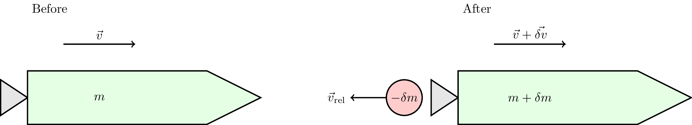
The initial momentum, which is conserved, is \(m \vec{v}\). The velocity of the exhaust gas is \(\vec{v}_\text{gas} = \vec{v} + \vec{v}_\text{rel}\), taking into account the relative velocity.
Conservation of momentum gives \[ m\vec{v} = (m + \delta m)(\vec{v} + \vec{\delta v}) + (-\delta m)(\vec{v} + \vec{v}_\text{rel}) \] Expanding and cancelling gives \[ \vec{0} = m\vec{\delta v} + \delta m \vec{\delta v} - \delta m \vec{v_\text{rel}} \] Dividing this by \(\delta t\) we get \[ \vec{0} = m \frac{\delta \vec{v}}{\delta t} + \frac{\delta m \vec{\delta v}}{\delta t} - \frac{\delta m}{\delta t} \vec{v_\text{rel}} \] Taking the limit at \(\delta t \to 0\), we can ignore second order terms like \(\delta m \delta \vec{v}\), to get
\[ m \frac{d\vec{v}}{dt} = \vec{v}_\text{rel} \frac{dm}{dt} \]
- \(m d\vec{v} / dt\) is the resultant thrust on the rocket,
- \(\vec{v}_\text{rel}\) is in the opposite direction to the rocket, and
- \(dm / dt < 0\),
so this makes sense.
A rocket burns 400,000 kg of fuel in 200 seconds, producing an average thrust of \(8 \times 10^6 \text{ N}\). What is the speed of the exhaust?
\[ \frac{dm}{dt} = \frac{400000}{200} = 2000 \text{ kg s}^{-1} \] The thrust is given by the rocket equation above \[ 8.6 \times 10^6 = v_\text{rel} \frac{dm}{dt} = v_\text{rel} \times 2000 \] \[ \implies v_\text{rel} = 4300 \text{ m s}^{-1} \]
We can now solve the rocket equation to get the velocity of the rocket. Gravity will oppose the thrust, and we can add this in as a constant vector \(\vec{g}\). In reality \(\vec{g}\) will vary with height, but for simplicity we’ll assume it is constant. We’re also neglecting air resistance. Using vectors, we have the following \[ m\frac{d\vec{v}}{dt} = \vec{v}_\text{rel} \frac{dm}{dt} + m \vec{g} \] We can integrate this to get the velocity of the rocket as a function of time \[ \int_{\vec{v_0}}^{\vec{v}} d\vec{v'} = \vec{v}_\text{rel} \int_{m_0}^m \frac{dm'}{m} + \vec{g} \int_0^t dt' \]
\[ \vec{v} - \vec{v_0} = \vec{v}_\text{rel} \left[ \log_e m' \right]_{m_0}^m + \vec{g} t \]
\[ \vec{v} = \vec{v_0} + \vec{v}_\text{rel} \log_e \left( \frac{m}{m_0} \right) + \vec{g} t \]
Let’s revisit the rocket example above. If the rocket started off with a mass \(m_0 = 5.5 \times 10^5 \text{ kg}\), what is its velocity after 200 seconds when the first stage burns out?
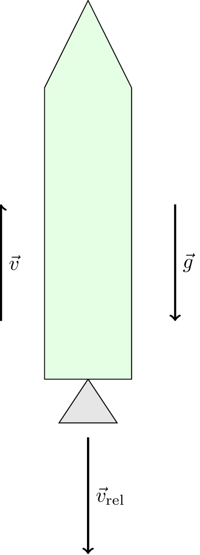
- The initial velocity is zero, \(\vec{v_0} = \vec{0}\).
- \(\vec{v}_\text{rel}\) and \(\vec{g}\) are in the negative direction.
- \(\vec{v}\) is in the positive direction.
This is illustrated in Figure 5.3.
The initial mass is \(m_0 = 5.5 \times 10^5 \text{ kg}\) but 400,000 kg of fuel have been burned. This means that the mass \[ m = 5.5 \times 10^5 - 4.0 \times 10^5 = 1.5 \times 10^5 \text{ kg}. \] We calculated above that \(| \vec{v}_\text{rel} = 4300 \text{ m s}^{-1}\). Using the rocket velocity equation and these values gives \[ v = 0 - 4300 \log_e \left( \frac{1.5}{5.5} \right) - 9.81 \times 200 \] \[ v = 3600 \text{ m s}^{-1} \]
5.4 Scalar product
I think this is a good time to have a mathematical interlude to consider the scalar product of two vectors. This is also known as the dot product. This takes two vectors and produces a scalar. It is a very useful operation in mechanics because it allows us to project vectors, e.g., forces, onto any direction specified by any unit vector.
So far, when resolving vectors (e.g., forces) we are used to projecting on the \(x\) and \(y\) axes (see Figure 5.4, in 2D). We can project these forces in the \(x\) and \(y\) directions as follows.
The components of \(\vec{f}\) in the \(x\) and \(y\) directions can be seen in vector form, \[ \vec{f} = f \cos \theta \hat{\imath} + f \sin \theta \hat{\jmath} \]
The components of \(m\vec{g}\) are \[ 0 \hat{\imath} - m|\vec{g}| \hat{\jmath} = -mg \hat{\jmath} \]
The components of \(\vec{B}\) are \[ -N \sin \theta \hat{\imath} + N \cos \theta \hat{\jmath} \]
However, we can project forces in any direction specified by any unit vector.
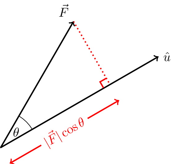
For example, in 2D, we can write the components of \(\vec{F}\) and unit vector \(\hat{u}\) relative to an arbitrary set of axes. The component of \(\vec{F}\) in the direction of \(\hat{u}\) is \(|\vec{F}| \cos \theta\) where \(\theta\) is the angle between \(\vec{F}\) and \(\hat{u}\), as shown in Figure 5.5.
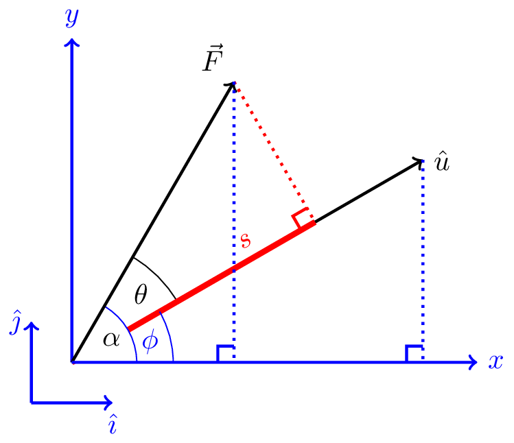
Using these axes, we have \[ \hat{u} = \cos\phi \hat{\imath} + \sin\phi \hat{\jmath}= \bar{u}_x \hat{\imath} + \bar{u}_y \hat{\jmath} \] \[ \vec{F} = F \cos\alpha \hat{\imath} + F \sin\alpha \hat{\jmath} = F_x \hat{\imath} + F_y \hat{\jmath} \]
Projecting \(\vec{F}\) onto \(\hat{u}\) gives a scalar, \(s\), \[ s = |\vec{F}| \cos\theta \]
From Figure 5.6 we can see that \(\theta = \alpha - \phi\) so \[ s = |\vec{F}| \cos(\alpha - \phi) \] which we can expand using a trigonometric identity to get \[ s = \left| \vec{F} \right| (\cos\alpha \cos\phi + \sin\alpha \sin\phi) \] \[ = F_x \bar{u}_x + F_y \bar{u}_y \]
We say that \(s\) is the scalar product (or dot product) of \(\vec{F}\) with unit vector \(\hat{u}\) \[ s = \vec{F} \cdot \hat{u} = |\vec{F}|\cos\theta = F_x \bar{u}_x + F_y \bar{u}_y \]
Geometrically, this is the projection of \(\vec{F}\) in the direction \(\hat{u}\).
More generally \[ \vec{F} \cdot \hat{u} = \frac{\vec{F} \cdot \vec{u}}{|\vec{u}|} \] from which we get \[ \vec{F} \cdot \vec{u} = |\vec{F}||\vec{u}|\cos\theta \]
The scalar product of any two vectors \(\vec{F}\) and \(\vec{u}\) in three dimensions is \[ \vec{F} \cdot \vec{u} = |\vec{F}||\vec{u}|\cos\theta = F_x u_x + F_y u_y + F_z u_z \] where \(\theta\) is the angle between \(\vec{F}\) and \(\vec{u}\).
Some special cases:
- The dot product of a vector with itself gives its magnitude squared \(\vec{a} \cdot \vec{a} = |\vec{a}||\vec{a}| \cos 0 = |\vec{a}|^2\).
- The dot product of two perpendicular vectors is zero. If \(\vec{a} \perp \vec{b}\) then \(\vec{a} \cdot \vec{b} = |\vec{a}||\vec{b}| \cos 90 = 0\).
5.5 Forces
In discussing golf balls and rockets we have already been considering contact forces and force fields. Now we’re going to look at these more carefully, and in more detail.
5.5.1 Contact forces
Contact forces act at a point on a body, generally due to contact with another part of the system. Typical examples of contact forces include the following.
- Friction acting between a sliding block and table.
- Tension in a rope.
- Push from a bat hitting a ball.
5.5.2 Force fields
Force fields generate forces that are a function of position (or velocity) only. Examples of force fields include the following.
- Force on a charge due to an electric field
- Gravitational force
The force on a charge \(q\) in an electric field \(\vec{E}(\vec{r})\) is given by \[ \vec{F}(\vec{r}) = q \vec{E}(\vec{r}) \] where \(\vec{r}\) is the position vector \[ \vec{r} = x \hat{\imath} + y \hat{\jmath} + z \hat{k} \].
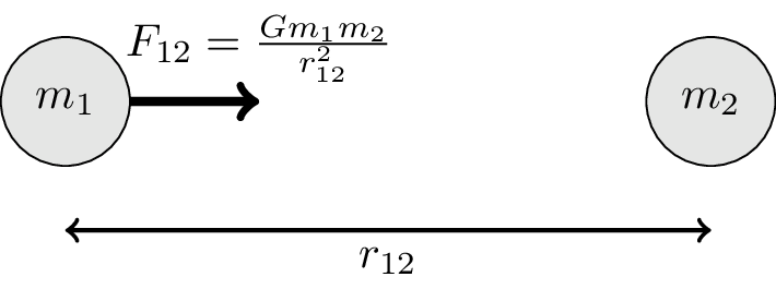
The force of one mass on another due to their gravitational field is given by \[ F_{12} = \frac{G m_1 m_2}{r_{12}} \] where \(r_{12}\) is the distance between the two masses. This is illustrated in Figure 5.7 which shows the force on \(m_1\) due to \(m_2\). The force on \(m_2\) due to \(m_1\) is equal and opposite. This is Newton’s law of gravity.
5.6 Statics
We’ll start by looking at some classic examples of statics problems where all of the forces are balanced so there is no net acceleration. This is also known as equilibrium. If we’re in an inertial frame in which the object is at rest, it will remain at rest. We have \[ \sum_i \vec{F}_i = \vec{0} \] where \(\vec{F}_i\) are the individual forces acting on the body.
5.6.1 Example 1: a block on a table
A stationary block on a table is shown in Figure 5.8. The forces acting on the block are the weight \(m\vec{g}\), the normal reaction force \(\vec{N}\), which must balance if there is no acceleration.
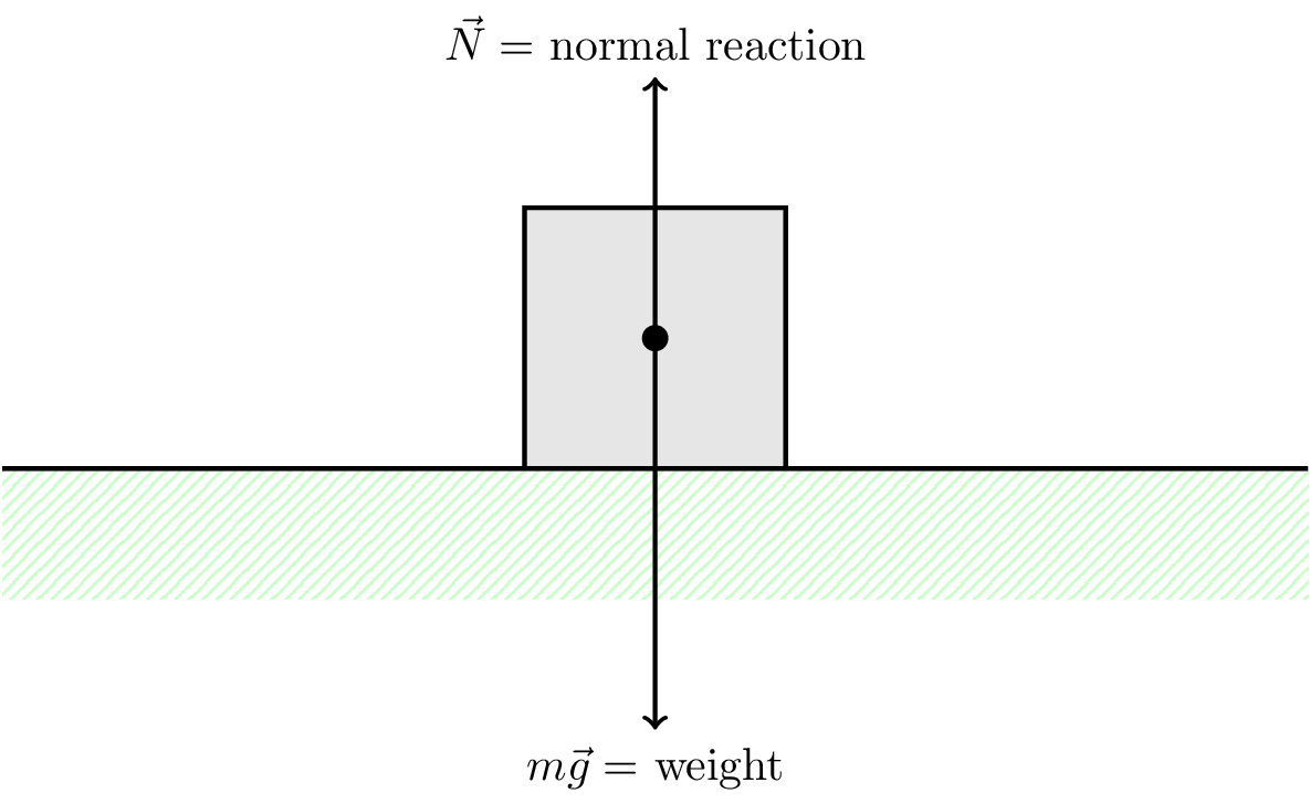
\[ \sum \vec{\text{forces}} = \vec{0} \] \[ m\vec{g} + \vec{N} = \vec{0} \] \[ m\vec{g} = -\vec{N}\] so the vectors \(\vec{g}\) and \(\vec{N}\) are antiparallel, with \(|\vec{N}| = m|\vec{g}|\).
5.6.2 Example 2: hanging a picture
A picture is hanging from two wires, as shown in Figure 5.9. Consider the forces acting through the centre of mass to avoid rotations (we’ll discuss rotations later). We will consider the downwards direction to be “positive”.
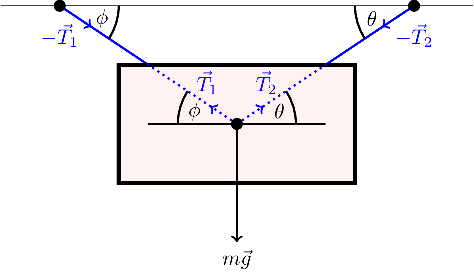
The sum of the forces acting on the frame must be zero. \[ m\vec{g} + \vec{T}_1 + \vec{T}_2 = \vec{0} \] where \(\vec{T}_1\) and \(\vec{T}_2\) are the tensions in the wires.
Consider the vertical component (obtained by taking the scalar product with \(\hat{\jmath}\)) \[ mg - T_1 \sin\phi - T_2 \sin\theta = 0 \tag{5.2}\] The horizontal component (obtained by taking the scalar product with \(\hat{\imath}\)) is \[ -T_1 \cos\phi + T_2 \cos\theta = 0 \tag{5.3}\]
We can eliminate \(T_2\) by taking (Equation 5.2) \(\times \cos\theta +\) (Equation 5.3) \(\times \sin\theta\) to get \[ mg\cos\theta - T_1\sin\phi\cos\theta - T_1\cos\phi\sin\theta =0 \] \[ T_1 = \frac{mg\cos\theta}{\sin\phi\cos\theta + \cos\phi\sin\theta} = \frac{mg\cos\theta}{\sin(\theta+\phi)} \]
Similarly, \[ T_2 = \frac{mg\cos\phi}{\sin(\theta+\phi)} \]
5.6.3 Example 3: tethered block on smooth plane
A block of mass \(m\) is tethered to a point on a smooth (frictionless) plane, as shown in Figure 5.10. The tension in the rope is \(\vec{T}\) and the normal reaction force is \(\vec{N}\).
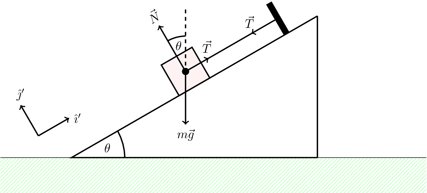
The block is static so is not accelerating, i.e,. \(\vec{a} = \vec{0}\). The sum of the forces acting on the block must therefore be zero, \[ m\vec{g} + \vec{N} + \vec{T} = \vec{0} \tag{5.4}\]
Note that we can choose coordinate axes parallel and perpendicular to the plane to simplify the maths. These coordinate unit vectors are shown in Figure 5.10 as \(\hat{\imath}'\) and \(\hat{\jmath}'\). In this coordinate system the individual force vectors are as follows. \[ m\vec{g} = -mg(\sin\theta \hat{\imath}' + \cos\theta \hat{\jmath}') \] \[ \vec{N} = N \hat{\jmath}' \] \[ \vec{T} = T \hat{\imath}' \]
Taking the scalar product of Equation 5.4 with \(\hat{\imath}'\) and \(\hat{\jmath}'\) gives the following scalar equations.
Parallel to the plane \[ -mg\sin\theta + T = 0 \] \[ \therefore T = mg\sin\theta \] Perpendicular to the plane \[ -mg\cos\theta + N = 0 \] \[ \therefore N = mg\cos\theta \]
This analysis is simpler than if we have used the coordinate axes \(\hat{\imath}\) and \(\hat{\jmath}\). These still work, which you can try to confirm.
5.7 Dynamics
When the net forces are not balanced we have a non-zero acceleration. \[ \sum \vec{\text{forces}} = m\vec{a} \] where \(\vec{a}\) is the resultant acceleration of the body.
5.7.1 Example 1: block on an inclined smooth plane
Consider a block on a smooth, inclined plane as shown in Figure 5.11. The block has mass \(m\) and the angle of the plane is \(\theta\). The block is accelerating down the plane with acceleration \(\vec{a}\).
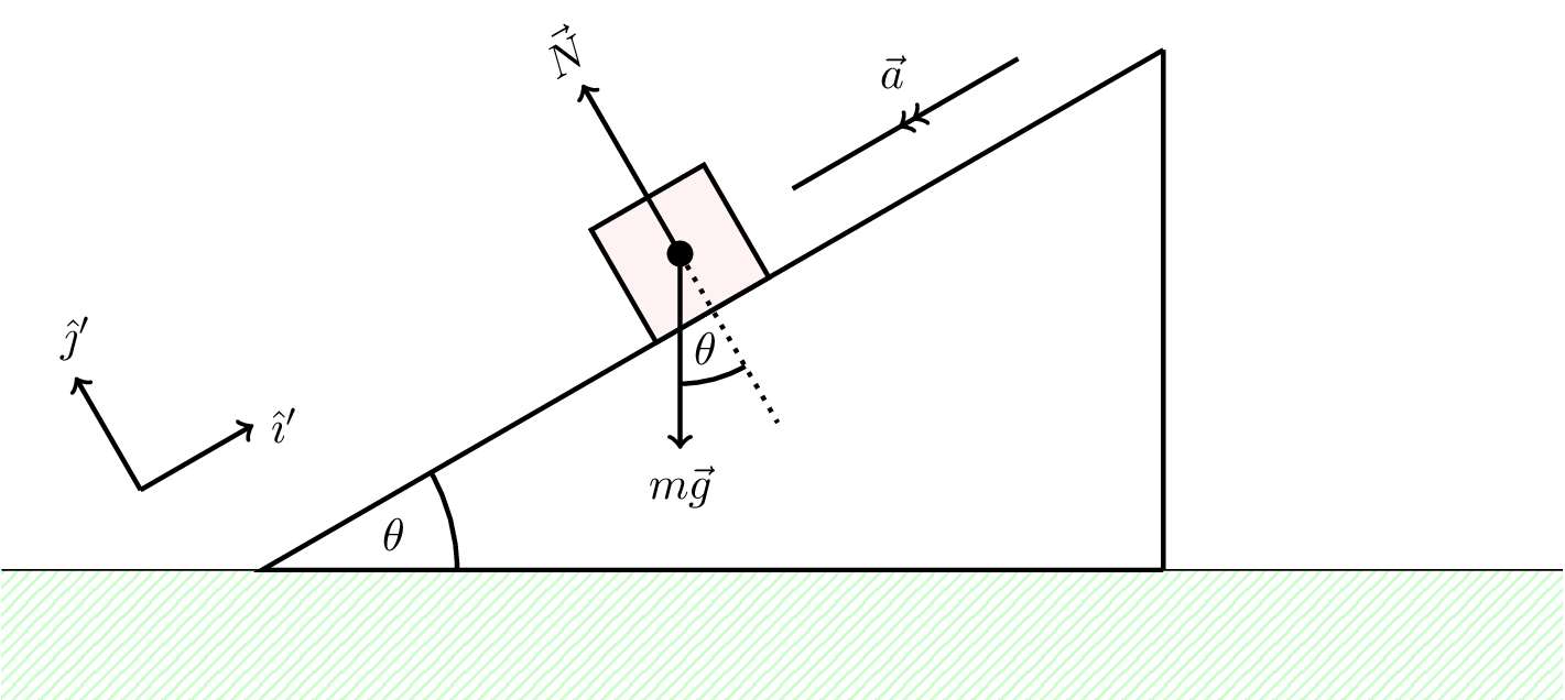
\[ \sum F_i = m\vec{g} + \vec{N} = m\vec{a} \] \[ -mg (\sin\theta \hat{\imath}' + \cos\theta \hat{\jmath}') + N \hat{\jmath}' = ma\hat{\imath}' \]
The component parallel to the plan can be found by taking the scalar product with \(\hat{\imath}'\), \[ -mg\sin\theta = ma \] \[ \therefore a = -g\sin\theta \] The component perpendicular to the plane can be found by taking the scalar product with \(\hat{\jmath}'\), \[ -mg\cos\theta + N = 0 \] \[ N = mg\cos\theta \]
The acceleration vector is \[ \vec{a} = -g\sin\theta\hat{\imath}' \]
5.7.2 Example 2: block and spring
Consider a block on a horizontal, smooth table attached to a spring, as shown in Figure 5.12.
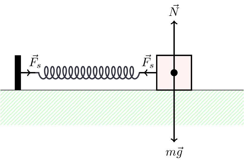
As ususal, \[ \vec{F}_s + \vec{N} + m\vec{g} = m\vec{a} \]
The vertically the forces balance so there is no acceleration in the vertical direction, i.e., \(\vec{N} = -m\vec{g}\).
Horizontally, \[ F_s = ma \]
The force provided by the spring is given by Hooke’s law, \[ F_s = - k x \] where \(k\) is the stiffness of the spring, and \(x\) is the extension of the spring. This gives us an equation of motion \[m \ddot{x} + kx = 0 \tag{5.5}\] where \(\ddot{x}\) is the second derivative of \(x\) with respect to time.
This is the equation of simple harmonic motion (more about that in the third part of this unit on Oscillations and Waves). Some of you will have seen this before, but don’t worry if you haven’t. You can verify by substitution that the following is a solution to this equation \[ x = x_0 \cos (\omega t) \] where \(x_0\) s the initial extension of the spring, and \[ \omega = \sqrt{\frac{k}{m}} \] is the angular frequency.
You should substitute this solution into Equation 5.5 to confirm.
5.8 Friction
Newton’s first law states that bodies only stop if a force acts. However, we experience things stopping all the time. We now know that this stopping is cause by friction.
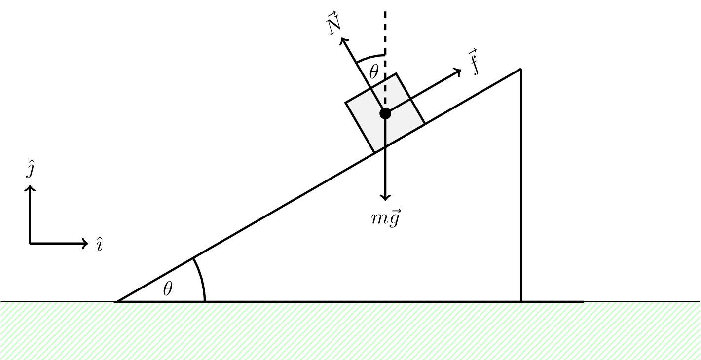
A classic example of friction is a block on a table. This is illustrated in Figure 5.13.
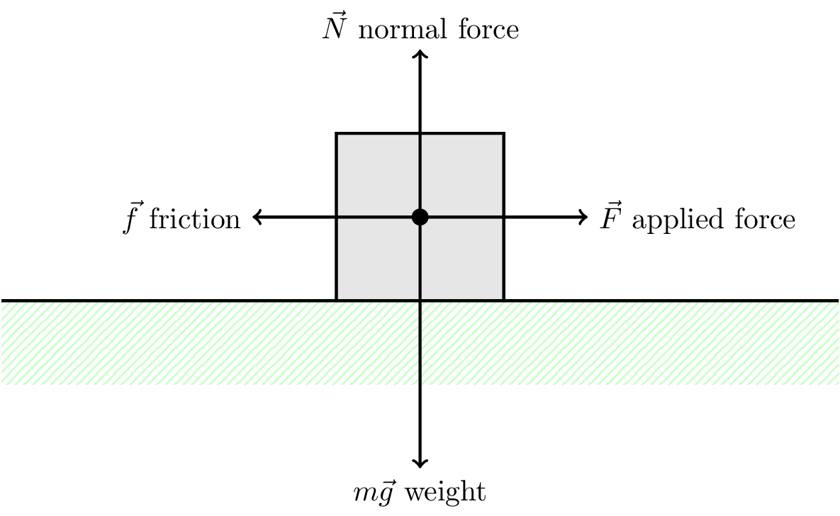
We can use Newton’s second law to write \[ \text{sum of forces acting} = \text{mass} \times \text{resultant acceleration of block} \] Using vector notation this can be written \[ \vec{f} + \vec{F} + m\vec{g} + \vec{N} = m\vec{a} \]
We can look at the horizontal and vertical components of the motion separately.
The horizontal, scalar components are \[ F - f = ma \] and the vertical components are balanced (no vertical acceleration) \[ N - mg = 0 \] \[ \therefore N = mg \]
The horizontal acceleration of the block will depend on the applied force and the friction force.
5.8.1 Coefficient of friction
The friction force is difficult to model in detail because it depends on the surface roughness and composition. However, in experiments we empirically observe that the friction force is proportional to the normal force, i.e. the force perpendicular to the surface.
\[ | \vec{f} | \propto | \vec{N} | \] In scalar notation \[ f = \mu N \] in scalars where \(\mu =\) coefficient of friction.
The friction force, \(\vec{f}\), acts to oppose the direction of motion that would occur in the absence of friction.
5.8.2 Kinetic friction
If the object is moving, the friction force is called kinetic friction. The coefficient of kinetic friction is denoted \(\mu_k\). This is also known as sliding friction. Consider a block sliding along a rough table as shown in Figure 5.14.
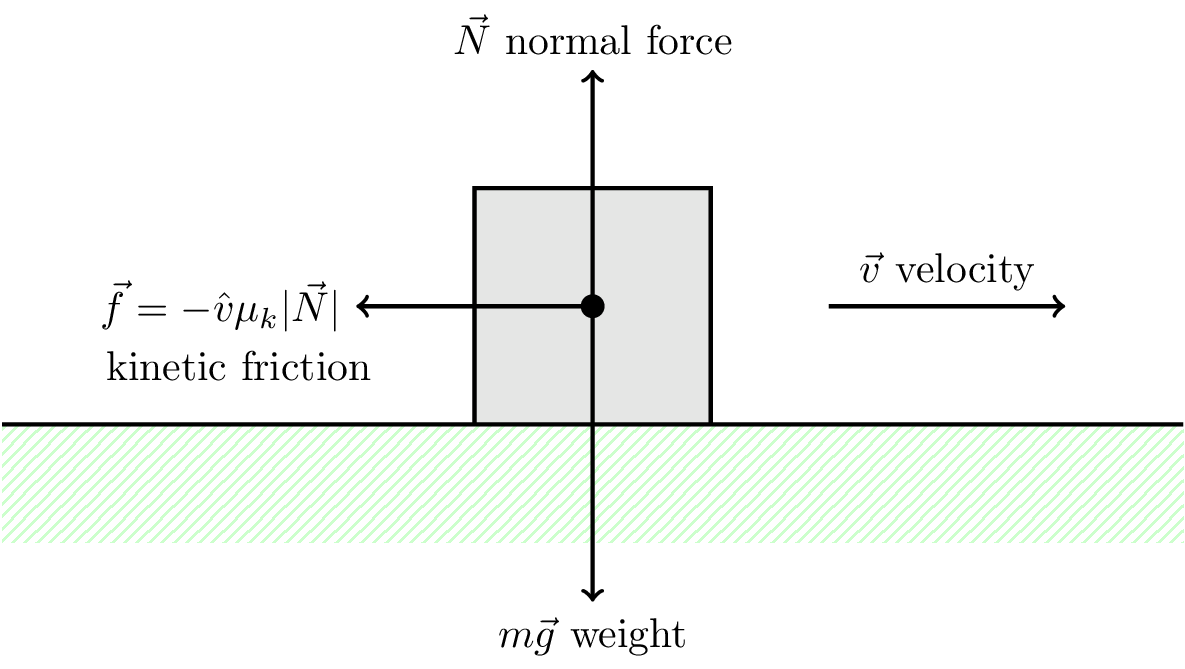
The friction force \(\vec{f}\) is given by \[ \vec{f} = -\hat{v} \mu_k | \vec{N} | \] where \(\hat{v}\) is the unit vector in the direction of motion, and \(| \vec{N} |\) is the magnitude of the normal reaction force. Notice that the friction force is in the opposite direction to the motion.
5.8.3 Static friction
If there is no net motion, the friction force is called static friction. The coefficient of static friction is denoted \(\mu_s\). This is also known as sticking friction. Consider a block on a rough table that is being pushed, but is not moving, as shown in Figure 5.15.
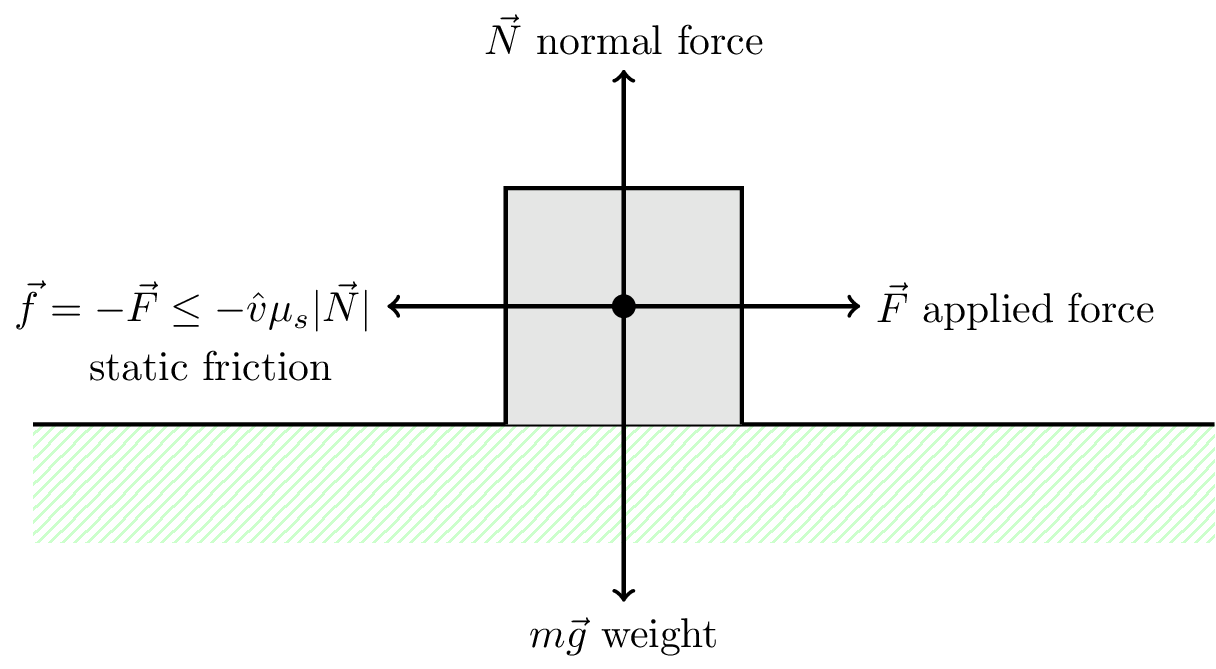
The friction force is given by \[ f \le \mu_s | \vec{N} | \]
As the applied force \(\vec{F}\) increases, the static friction force will also increase to balance it, i.e., \(\vec{f} = -\vec{F}\). The friction force can increase to the limit \(f = \mu_s | \vec{N} |\), beyond which the block will start to move, where the friction force is then equal to the (lower) kinetic friction force \(f = \mu_k | \vec{N} |\).
In practice, \(0 < \mu_k < \mu_s < 1\).
Typical values of \(\mu_s\) and \(\mu_k\) are given in Table 5.1.
| Surface | \(\mu_s\) | \(\mu_k\) |
|---|---|---|
| Rubber on concrete | 1.0 | 0.8 |
| Steel on steel | 0.7 | 0.6 |
| Waxed ski | 0.1 | 0.05 |
5.8.4 Drag
Friction due to motion through a fluid, gas or liquid is called drag. This is a major topic in fluid mechanics. The drag direction opposes the motion \(\hat{f} = -\hat{v}\), as shown in Figure 5.16.
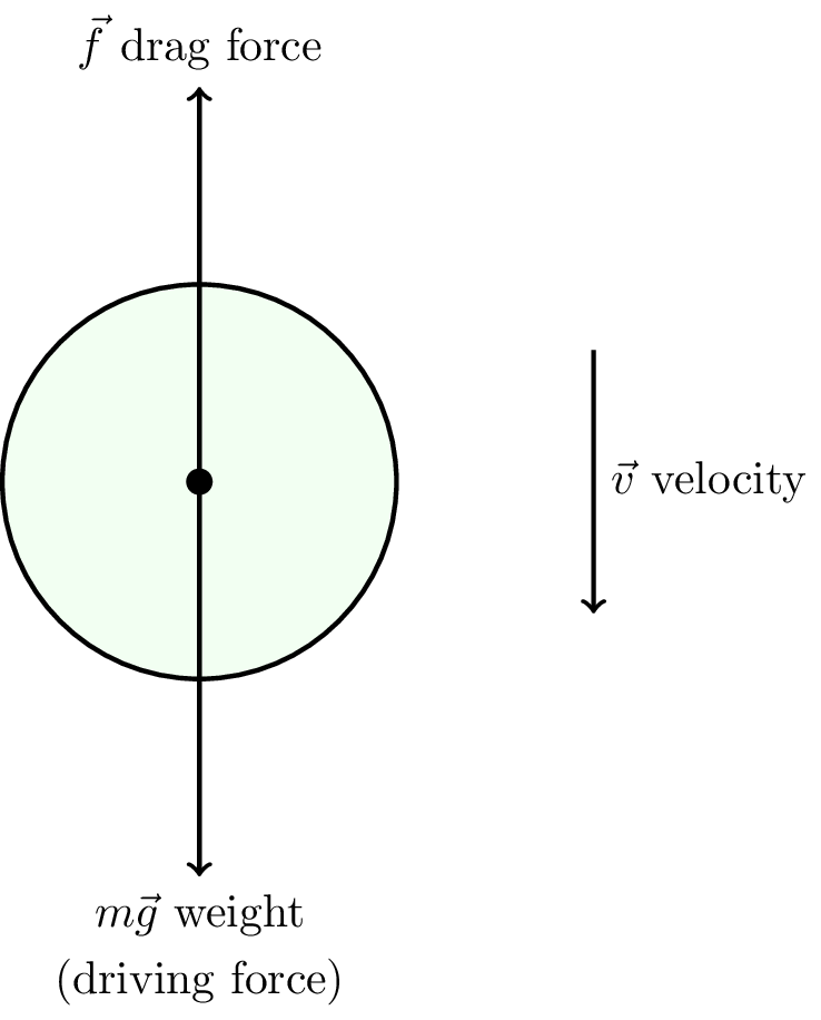
Generally \[ | \vec{f} | \propto | \vec{v} |^n \]
- \(n = 1\) for microscopic particles in water.
- \(n = 1\) for human swimming in treacle.
- \(n = 2\) for free-falling through the atmosphere.