8 Rotational mechanics
Before getting into rotational mechanics properly, we’ll first introduce the idea of the cross product or vector product because that will turn out to be particularly useful in our description of rotational motion and angular momentum in particular.
8.1 Cross product
Earlier in the course we looked at the scalar product that takes two vectors and produces a scaler. We are now going to introduce something called the vector product, or cross product, which takes two vectors and produces a third vector.
For a geometrical interpretation of the cross product, consider two vectors \(\vec{a}\) and \(\vec{b}\), with an angle \(\theta\) between them, as shown in Figure 8.1. The area of the parallelogram with these vectors as sides is \(A = |\vec{a}| |\vec{b}| \sin \theta\). We can use this to define a vector that is in the direction perpendicular to the plane containing \(\vec{a}\) and \(\vec{b}\), and has a magnitude equal to the area of the parallelogram. The direction of this vector is chosen to produce a right-handed set of vectors. This is the cross product of \(\vec{a}\) and \(\vec{b}\), written \(\vec{a} \times \vec{b}\).

The cross product of two vectors \(\vec{a}\) and \(\vec{b}\) is defined as \[ \vec{a} \times \vec{b} = |\vec{a}| |\vec{b}| \sin \theta \hat{n} \] where \(\theta\) is the angle between the vectors, and \(\hat{n}\) is a unit vector perpendicular to \(\vec{a}\) and \(\vec{b}\) that forms a right-handed set of vectors.
Note: if \(\vec{a}\) and \(\vec{b}\) are parallel, \(\vec{a} \times \vec{b} = \vec{0}\).
Also, because of the need for the right handed set of vectors, \(\vec{a} \times \vec{b} = - \vec{b} \times \vec{a}\). We say that the vector product is non-commutative, i.e., the order of the vectors matters.
We can determine the components of the cross product by considering the cross product of units vectors in a cartesian coordinate system, which is right-handed (see Figure 8.2).
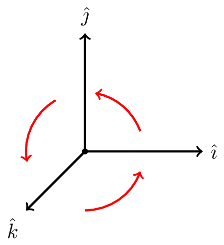
\[ \hat{\imath} \times \hat{\jmath} = \hat{k} \] \[ \hat{\jmath} \times \hat{k} = \hat{\imath} \] \[ \hat{k} \times \hat{\imath} = \hat{\jmath} \]
And similarly, \(\hat{\jmath} \times \hat{\imath} = - \hat{k}\), \(\hat{k} \times \hat{\jmath} = - \hat{\imath}\), and \(\hat{\imath} \times \hat{k} = - \hat{\jmath}\).
Since the cross product of parallel vectors is zero, we also note that \(\hat{\imath} \times \hat{\imath} = \hat{\jmath} \times \hat{\jmath} = \hat{k} \times \hat{k} = \vec{0}\).
The vector product is distributive, which means that \[ \vec{a} \times ( \vec{b} + \vec{c} ) = \vec{a} \times \vec{b} + \vec{a} \times \vec{c} \] but it is not associative, which means that \[ \vec{a} \times ( \vec{b} \times \vec{c} ) \neq ( \vec{a} \times \vec{b} ) \times \vec{c} \] so when you are writing cross products with three vectors like this the brackets are important. As a concrete example that illustrates this, consider the difference between \(\hat{\imath} \times (\hat{\imath} \times \hat{j})\) and \((\hat{\imath} \times \hat{\imath} ) \times \hat{j}\).
We can now determine the cross product of arbitrary vectors as follows. \[ \vec{a} \times \vec{b} = (a_x \hat{\imath} + a_y \hat{\jmath} + a_z \hat{k}) \times (b_x \hat{\imath} + b_y \hat{\jmath} + b_z \hat{k}) \] which we can multiply out and use the above properties of the basis unit vectors to get
\[ \vec{a} \times \vec{b} = (a_y b_z - a_z b_y)\hat{\imath} + (a_z b_x - a_x b_z)\hat{\jmath} + (a_x b_y - a_y b_x)\hat{k} \] Note the pattern of cyclic permutations. This can also be visualised graphically as shown below. 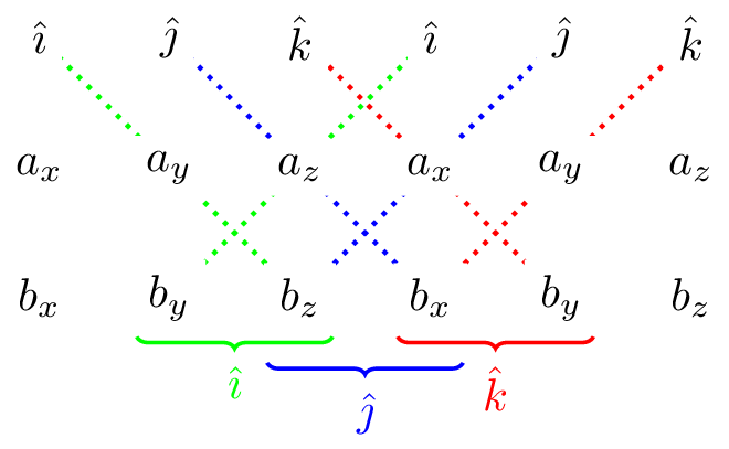
8.2 Circular motion
Circular motion is produced by a constant net force that is perpendicular to a particle’s velocity.
8.2.1 Position
If a particle is moving around a circle at constant speed (but not constant velocity because its direction is continuously changing), then we can write its coordinates at time \(t\) as: \[ x = r_0 \cos (\omega t) \] \[ y = r_0 \sin (\omega t) \] where \(r\) is the radius of the circle and \(\omega\) is the angular velocity of the particle. This is illustrated in Figure 8.3, where \(\phi = \omega t\).
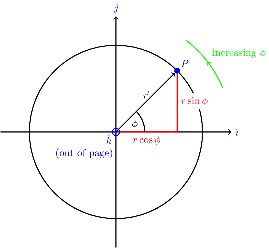
We can write this as a vector, \[ \vec{r} = r_0 ( \cos (\omega t) \hat{\imath} + \sin (\omega t) \hat{\jmath} ) \]
8.2.2 Velocity
The angular velocity is \(\dot{\phi}\), the rate of change of the angle \(\phi\) with time, \[ \dot{\phi} = \frac{d\phi}{dt} = \frac{d}{dt} (\omega t) = \omega \]
The angular velocity \(\omega\) is related to the period of the motion, \(T\) (the time to go once around the circle), by \[ \omega = \frac{2\pi}{T} \] with units of radians per second.
In terms of frequency, \(f\), \[ \omega = 2 \pi f \]
The particle travels a distance equal to the circumference of the circle (\(2\pi r_0\)) in one period (\(T\)), so the speed of the particle is \[ v = \frac{2\pi r_0}{T} = 2\pi r_0 \times \frac{\omega}{2\pi} = r_0 \omega \]
Another way to calculate the velocity of the particle is to differentiate its position with respect to time \[ \vec{v}(t) = \frac{d\vec{r}}{dt} = -r_0 \omega \sin(\omega t) \hat\imath + r_0 \omega \cos (\omega t) \hat\jmath \]
This is a directed tangentially. The speed is given by \[ v^2 = |\vec{v}|^2 = r_0^2 \omega^2 \underbrace{(\sin^2(\omega t) + \cos^2(\omega t))}_{\color{blue} 1} \] So, as before, \[ v = r_0 \omega \tag{8.1}\]
Note: \(\vec{v} \cdot \vec{r} = 0\), so the velocity and position vectors are perpendicular.
8.2.3 Acceleration
We find the acceleration by differentiating the velocity with respect to time. \[ \vec{a}(t) = \frac{d\vec{v}}{dt} = -r_0 \omega^2 \cos(\omega t) \hat{\imath} - r_0 \omega^2 \sin (\omega t) \hat{\jmath} \] \[ \vec{a}(t) = -r_0 \omega^2 \underbrace{(\cos(\omega t) \hat{\imath} + \sin(\omega g) \hat{\jmath})}_{\color{blue} \text{radial unit vector, } \hat{r}} \] \[ \vec{a}(t) = -r_0 \omega^2 \hat{r} \]
Hence the centripetal acceleration, \(a\), is given by \[ a = r_0 \omega^2 = \frac{v^2}{r_0} \]
The centripetal force is similarly \[ F = mr_0 \omega^2 = \frac{mv^2}{r_0} \]
Both the force and acceleration are directed towards the centre of the circle. \[ \vec{F} = -mr_0 \omega^2 \hat{r} = - \frac{mv^2}{r_0} \hat{r} \]
Note: Since \(\vec{v} \cdot \vec{F}_\text{cent} = 0\), a centripetal force does no work.
8.3 Angular velocity vector
We can combine the work of the previous two sections to write the angular velocity as a vector. This is useful because it tells us the axis of rotation, and will be useful for rotational mechanics in general.
We therefore choose the axis of rotation to define the direction of our angular velocity and use the cross product to define angular velocity vector as follows.
\[ \vec{\omega} = \frac{\vec{r} \times \vec{v}}{r^2} \tag{8.2}\] This is a vector that is perpendicular to the plane of the particle’s motion, and points in the direction of the axis of rotation.
Note: because this is a vector product the order of the terms is important to get the direction right.
For circular motion with angular velocity \(\omega\), \[ |\vec{v}| = r \omega \] in a direction perpendicular to \(\vec{r}\). This means that \[ \vec{\omega} = \omega \hat{n} \] where \(\hat{n}\) is a unit vector in the direction of the axis of rotation.
8.4 Angular acceleration vector for circular motion
This section only applies to circular motion, i.e., when \(\hat{\omega}\) is fixed but \(|\omega|\) is changing. The angular acceleration \(\vec{\alpha}\) is the time derivative of \(\vec{\omega}\).
\[ \vec{\alpha} = \frac{d\vec{\omega}}{dt} = \frac{d}{dt} \left( \frac{\vec{r} \times \vec{v}}{r^2} \right) \] For circular motion the radius \(r\) is constant (i.e., \(dr/dt = 0\)). \[ = \frac{1}{r^2} \left( \frac{d\vec{r}}{dt} \times \vec{v} + \vec{r} \times \frac{d\vec{v}}{dt} \right) \] \[ = \frac{1}{r^2} \left( \underbrace{\vec{v} \times \vec{v}}_{\color{blue} \vec{0}} + \vec{r} \times \vec{a} \right) \]
\[ \vec{\alpha} = \frac{\vec{r} \times \vec{a}}{r^2} \tag{8.3}\] Note: this only applies for circular motion.
Note that \(\vec{\alpha}\) is zero if the circular motion is at constant speed.
Assume the circular motion is not at constant speed. In scalars, we can write \(v = r \omega.\) Differentiating this gives the acceleration in the tangential direction, \(a_t = r \frac{d\omega}{dt}\). We arrive the following expression. \[ r |\vec{\alpha}| = r \times \frac{r \times r \frac{d\omega}{dt}}{r^2} = a_t \] where \(a_t\) is the acceleration in the tangential direction.
8.5 Torque and moment of inertia
Torque is the rotational analogue of force. It is also known as the moment of force.
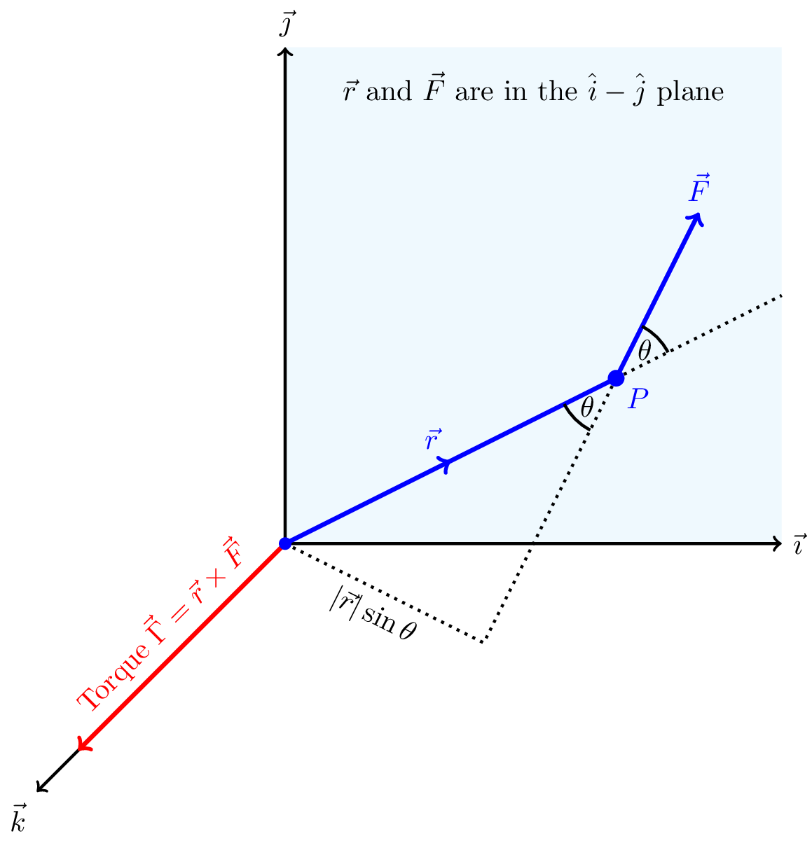
Torque is a vector quantity, \(\vec{\Gamma}\), defined as follows \[ \vec{\Gamma} = \vec{r} \times \vec{F} \tag{8.4}\] Where \(\vec{r}\) is the vector from the origin to the point at which the force \(\vec{F}\) is being applied. It is perpendicular to both \(\vec{r}\) and \(\vec{F}\), and points in the direction of the axis of rotation.
The magnitude of the torque is given by \[ |\vec{\Gamma}| = |\vec{r}| |\vec{F}| \sin \theta \] where \(\theta\) is the angle between \(\vec{r}\) and \(\vec{F}\). In other words, it is the perpendicular component of the force times the distance from the axis of rotation.
An illustration of torque is shown in Figure 8.4.
The units of torque are newton metres (Nm).
8.5.1 Circular motion
We can find an analogue to Newton’s second law by noting that \[ \vec{\Gamma} = \vec{r} \times \vec{F} = \vec{r} \times m \vec{a} \] Comparing this with Equation 8.3 we see that for circular motion the torque can be written as follows.
For circular motion we find the following relationship between torque, \(\vec{\Gamma}\), and angular acceleration, \(\vec{\alpha}\), \[ \vec{\Gamma} = mr^2 \vec{\alpha} \tag{8.5}\] where \(r\) is the radius of the circle. for a point particle of mass \(m\) a distance \(r\) from the rotation axis.
This is the rotational analogue to Newton’s second law. The torque is proportional to the angular acceleration, but the constant is not \(m\), rather it is \(mr^2\) which implies the distance of the particle from the rotation axis will affect its ability to increase the angular velocity.
8.5.2 Torque on a rigid body
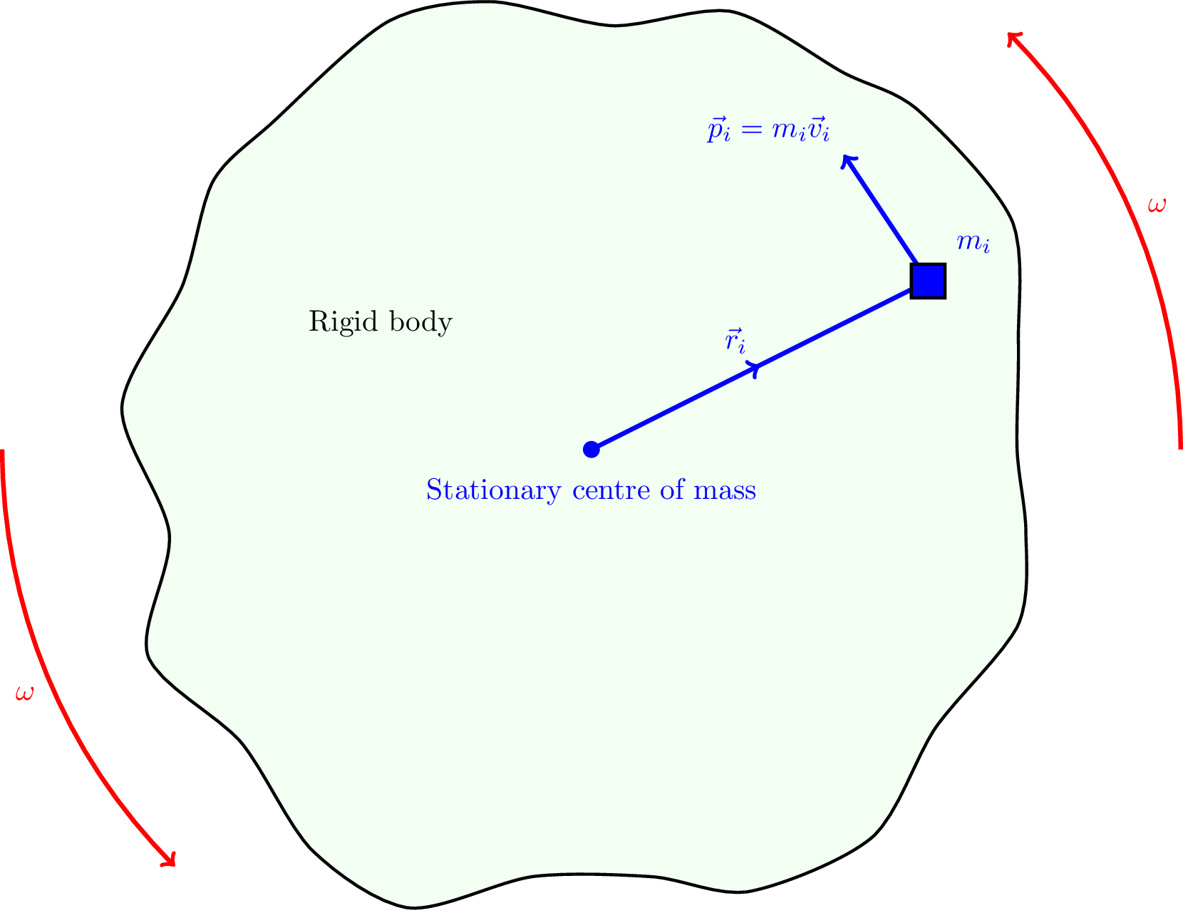
Consider a rigid body made up of \(N\), a large number, of individual masses \(m_1\), \(m_2\), \(\ldots\), at positions \(\vec{r}_1\), \(\vec{r}_2\), \(\ldots\), each acted upon by forces \(\vec{F}_1\), \(\vec{F}_2\), \(\ldots\). This is a rigid body so the distances between the masses are fixed and there is a single angular velocity vector \(\vec{\omega}\). The origin is placed at the centre of rotation, as shown in Figure 8.5, which need not be the centre of mass.
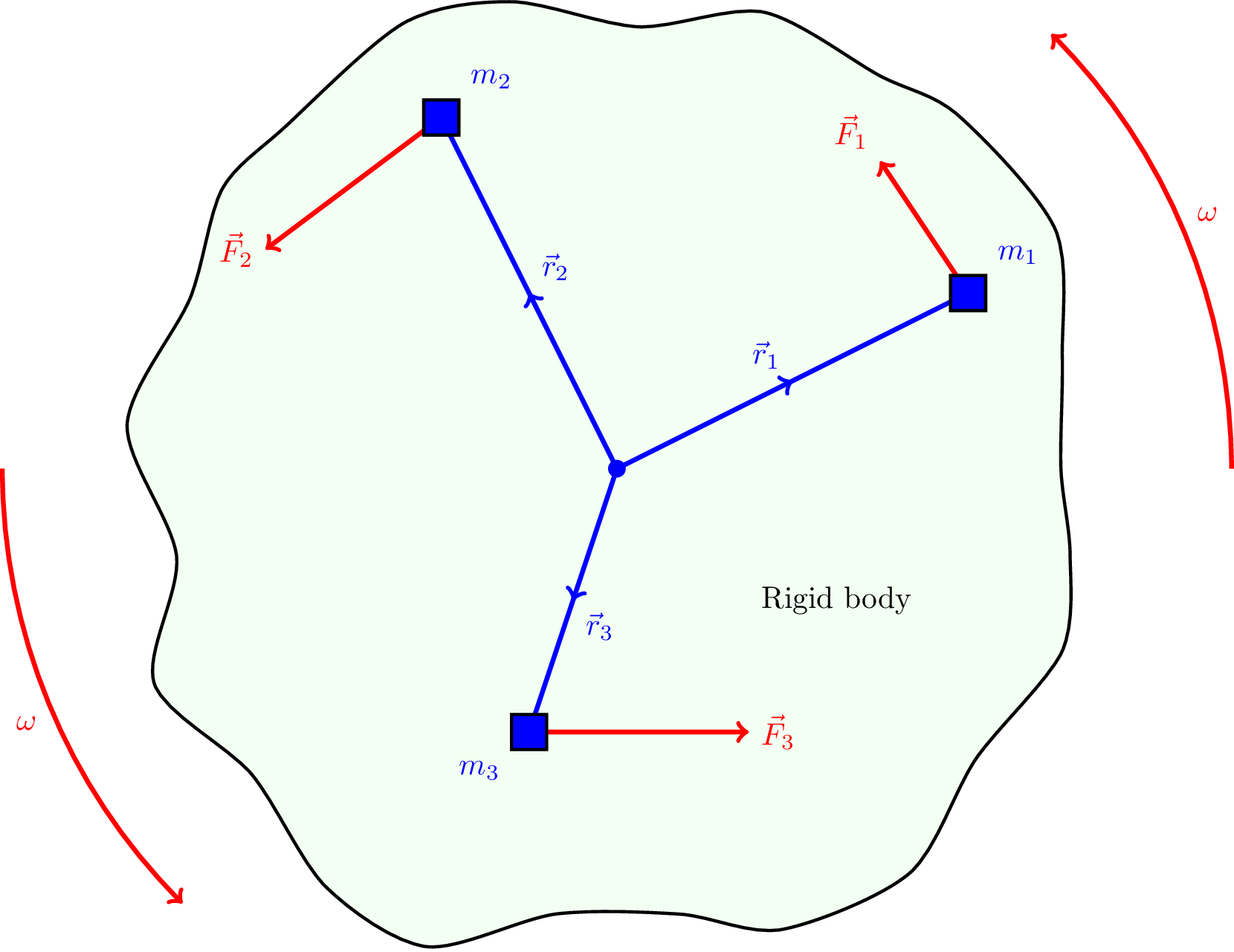
The torque acting on each individual mass is given by \[ \vec{\Gamma}_i = \vec{r}_i \times \vec{F}_i \] which, looking at Equation 8.5, is equivalent to \[ \vec{\Gamma}_i = m_i r_i^2 \vec{\alpha} \] where \(\vec{\alpha}\) is the same for each mass because this is a rigid body.
The total torque is the sum of each individual torque, noting that for a rigid body \(\vec{\alpha}\) is the same for each element, \[ \vec{\Gamma}_\text{tot} = \sum_{i=1}^N \vec{\Gamma}_i = \sum_{i=1}^{N} m_i r_i^2 \vec{\alpha} = \vec{\alpha} \sum_{i=1}^{N} m_i r_i^2 \]
8.5.3 Moment of inertia
This leads us to the following definition of the moment of inertia of a rigid body.
The moment of inertia, \(I\), of a rigid body is defined as follows \[ I = \sum_{i=1}^{N} m_i r_i^2 \tag{8.6}\] where \(m_i\) is the mass of the \(i\)th element of the body, and \(r_i\) is the distance of that element from the axis of rotation.
Moment of inertia has units of kg m\(^2\).
The total torque \(\vec{\Gamma}_\text{tot}\) on a rigid body is related to its angular acceleration \(\vec{\alpha}\) by \[ \vec{\Gamma}_\text{tot} = I \vec{\alpha} \] where \(I\) is the moment of inertia of the rigid body (Equation 8.6).
The role of \(I\) in rotational dynamics is analogous to \(m\) in linear dynamics, i.e., it resists angular acceleration.
If the torques balance, \(\vec{\Gamma} = \vec{0}\) and there is no change in angular velocity.
Consider a system that is balanced so there is no net torque about the origin, as shown in Figure 8.6.
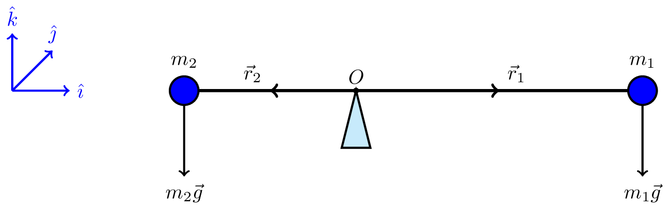
Using the right handed coordinate system shown in blue in the figure, we can write the radii and forces as follows. \[ \vec{r}_1 = r_1 \hat{\imath} \] \[ \vec{r}_2 = -r_2 \hat{\imath} \] \[ \vec{F}_1 = m_1 \vec{g} = -m_1 g \hat{k} \] \[ \vec{F}_2 = m_2 \vec{g} = -m_2 g \hat{k} \] The torques of the two particles are then obtained by using \(\vec{\Gamma}_i = \vec{r}_i \times \vec{F}_i\) as follows \[ \vec{\Gamma}_1 = r_1 \hat{\imath} \times (-m_1 g \hat{k}) = -m_1 g r_1 (\hat{\imath} \times \hat{k}) = m_1 g r_1 \hat{\jmath} \] \[ \vec{\Gamma}_2 = -r_2 \hat{\imath} \times (-m_2 g \hat{k}) = m_2 g r_2 (\hat{\imath} \times \hat{k}) = -m_2 g r_2 \hat{\jmath} \]
If the system is balanced the sum of these moments is zero \[ \vec{\Gamma}_1 + \vec{\Gamma}_2 = \vec{0} \] \[ m_1 g r_1 - m_2 g r_2 = 0 \] \[ m_1 r_1 = m_2 r_2 \]
This is an example of the principle of moments.
Here we calculate the moment of inertia of a ring about an axis perpendicular to the plane of the ring, passing through its centre.
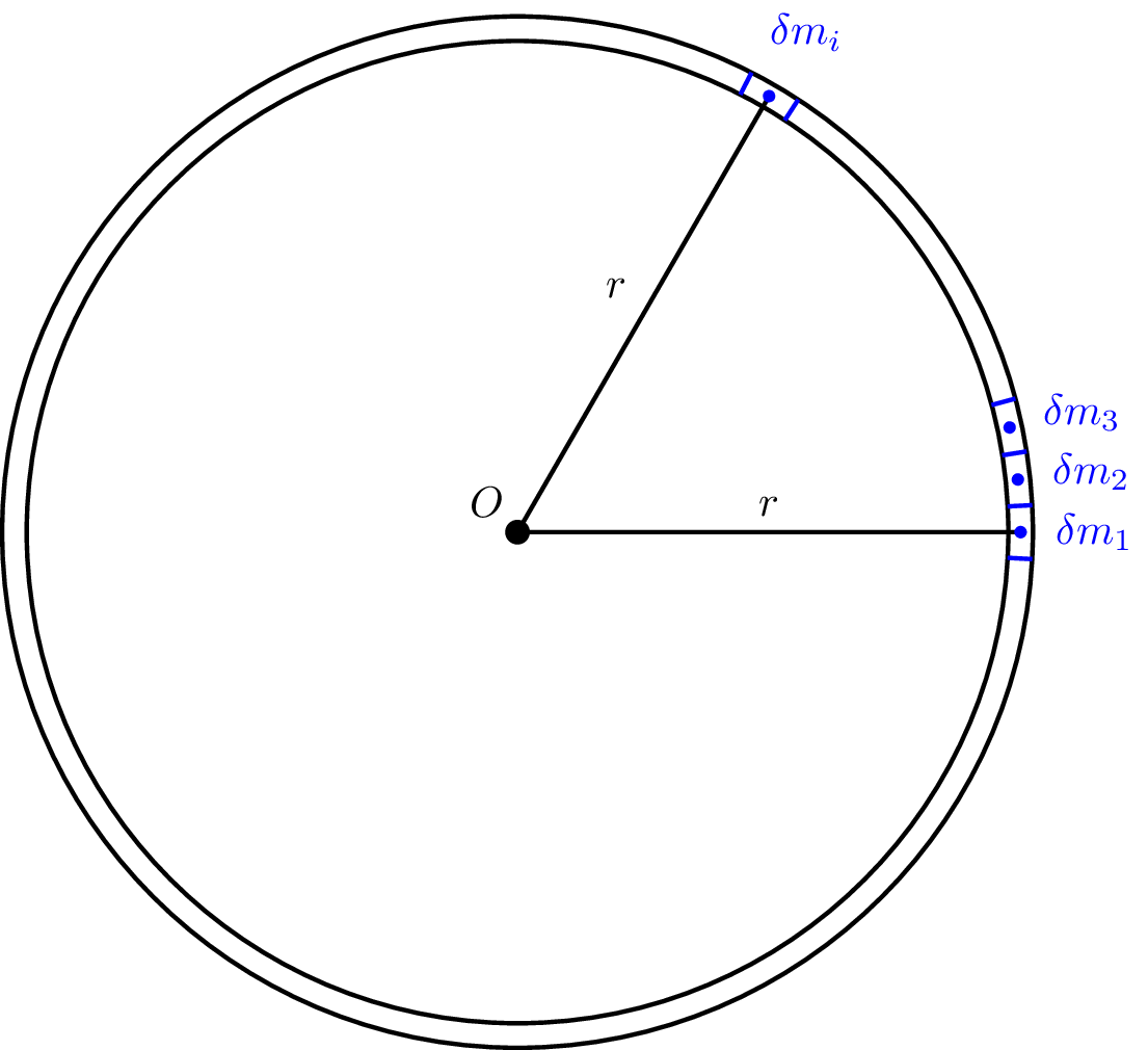
The ring can be thought of as a collection of little masses \(\delta m_i\) at equal distances \(r\) from centre, as shown in Figure 8.7. The moment of inertia is given by \[ I = \sum_i \delta m_i r^2 \] But the \(\sum_i \delta m_i = M\) where \(M\) is the total mass of the ring.
We therefore find that for a ring, the moment of inertia, \(I\), is given by \[ I = Mr^2 \] about an axis through \(0\) perpendicular to the plane of the ring.
8.6 Angular momentum
By analogy with torque, angular velocity, etc. we define for a particle with linear momentum \(\vec{p}\), the angular momentum \(\vec{L}\) as follows.
\[ \vec{L} = \vec{r} \times \vec{p} \tag{8.7}\] where \(\vec{r}\) is the vector from the origin to the particle, and \(\vec{p}\) is the linear momentum of the particle. This is illustrated in Figure 8.8.
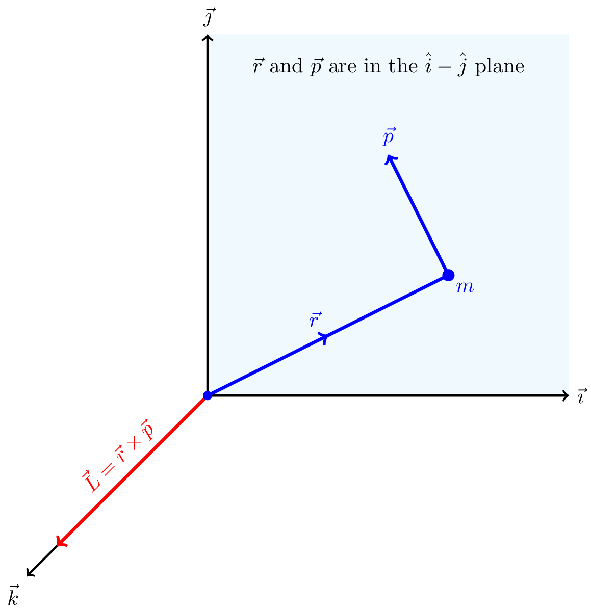
For circular motion \(\vec{r}\) and \(\vec{v}\) are perpendicular, so \(\vec{r}\) and \(\vec{p}\) are perpendicular. \[ |\vec{L}| = mvr \sin(90) = mvr = mr^2\omega \]
8.6.1 Angular momentum of a rigid body
Again we can consider splitting the body up into individual elements of mass \(m_i\) and momentum \(\vec{p}_i\) (similar to what we did for torque, as illustrated by Figure 8.5).
The total angular momentum is then the sum of the angular momenta of the individual elements. I.e., \[ \vec{L}_\text{tot} = \sum_{i=1}^N \vec{r}_i \times \vec{p}_i \] \[ = \sum_i \vec{r}_i \times m_i \vec{v}_i \] Recall (Equation 8.2) that \(\vec{\omega} = \frac{\vec{r} \times \vec{v}}{r^2}\), so we can write \[ \vec{L}_\text{tot} = \sum_i m_i r_i^2 \vec{\omega} \] \(\vec{\omega}\) is the same for each element because it is a solid body, and \(\sum_i m_i r_i^2\) is the moment of inertia, \(I\). Hence we find that
\[ \vec{L} = I \vec{\omega} \] where \(I\) is the moment of inertia of the rigid body, and \(\vec{\omega}\) is the angular velocity of the rigid body.
8.6.2 Conservation of angular momentum
Angular momentum is conserved separately from linear momentum.
Just as force rate of change of linear momentum so torque is the rate of change of angular momentum. Looking at Equation 8.7 (\(\vec{L} = \vec{r} \times \vec{p}\)), Equation 8.4 (\(\vec{\Gamma} = \vec{r} \times \vec{F}\)), and considering Newton’s second law Equation 5.1 (\(\vec{F} = d\vec{p}/dt\)), we see that \[ \vec{\Gamma} = \frac{d\vec{L}}{dt} \]
This immediately shows that if there is no net torque on a system then the total angular momentum is conserved.
As a rope wraps around pole its horizontal distance from the pole decreases from \(r_1\) to \(r_2\), as shown in Figure 8.9.
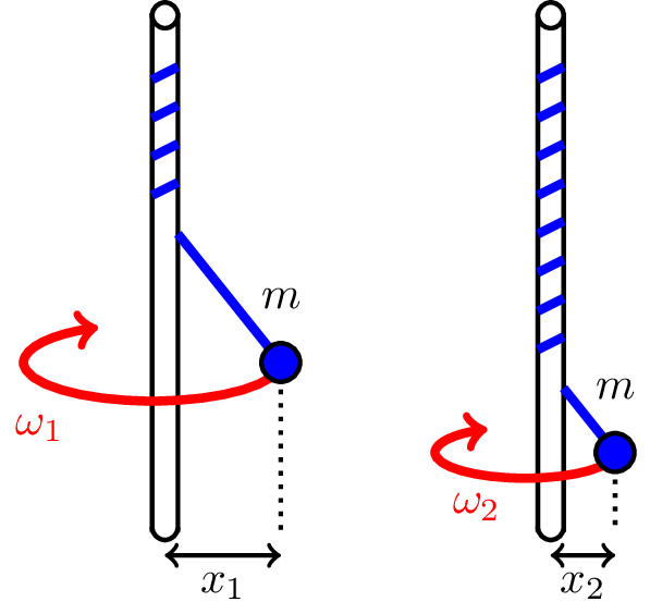
The initial and final moments of inertia of the mass about the pole are \[ I_1 = mr_1^2 \] \[ I_2 = mr_2^2 \] The corresponding expressions for angular momentum are \[ L_1 = I_1 \omega_1 \] \[ L_2 = I_2 \omega_2 \] Angular momentum is conserved so \(L_1 = L_2\) which implies \[ I_1 \omega_1 = I_2 \omega_2 \] \[ \omega_2 = \frac{I_1}{I_2} \omega_1 \] Since \(I_1 > I_2\) we find that \(\omega_2 > \omega_1\) and the rotational frequency increases.
8.7 Rotational kinetic energy
Consider a rigid body rotating freely about its centre of mass, shown in Figure 8.10. As before, we can consider splitting the body into \(N\) elements of mass \(m_i\), each with momentum \(\vec{p}_i\). The total kinetic energy is the sum of the kinetic energies of the individual elements.
The total rotational kinetic energy is then \[ \text{KE}_\text{rot} = \sum_{i=1}^N \frac{1}{2} m_i v_i^2 \] But \(v_i = r_i \omega\) (Equation 8.1), so \[ \text{KE}_\text{rot} = \sum_{i=1}^N \frac{1}{2} m_i r_i^2 \omega^2 \] and we have just shown (Equation 8.6) that \(I = \sum_i m_i r_i^2\). This gives us an expression for the rotational kinetic energy in terms of the moment of inertia and the angular velocity.
\[ \text{KE}_\text{tot} = \frac{1}{2} I \omega^2 \] where \(I\) is the moment of inertia of the rigid body, and \(\omega\) is the angular velocity of the rigid body.
A rigid body carries kinetic energy in two forms:
- linear KE through centre of mass motion and
- rotational KE about the centre of mass.
\[ \text{KE}_\text{tot} = \frac{1}{2} Mv_\text{com}^2 + \frac{1}{2} I \omega^2 \] where \(M\) is the total mass of the rigid body, \(v_\text{com}\) is the velocity of the centre of mass, \(I\) is the moment of inertia of the rigid body about the centre of mass, and \(\omega\) is the angular velocity.
8.8 Conservation of mechanical kinetic energy
When conserving mechanical energy all forms of energy should be considered
- Potential energy
- Linear KE
- Rotational KE
- Linear work
- Rotational work
8.8.1 Rotational work
Consider a force \(\vec{F}\) producing a torque \(\vec{\Gamma}\) resulting in a small angular change \(d\theta\), as shown in Figure 8.11.
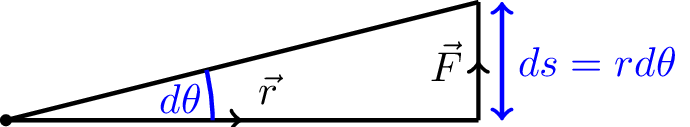
For small \(d\theta\) the displacement will be \(ds = r d\theta\) and the work done will be \(dW = F ds = F r d\theta = \Gamma d\theta\).
We can integrate \(dW\) to find the work done for a large angular rotation.
Consider constant torque acting to rotate a body from an angle \(\theta = \theta_0\) to \(\theta = \theta_1\).
The rotational work is equal to the constant torque times the angle moved through.
\[ \text{Rotational work} = \int_{\theta_0}^{\theta_1} \Gamma d\theta = \int_{\theta_0}^{\theta_1} I\alpha d\theta \].
Using the chain rule we can write \[ \alpha = \frac{d\omega}{dt} = \frac{d\omega}{d\theta} \frac{d\theta}{dt} = \omega \frac{d\omega}{d\theta} \] Therefore \[ \text{Rotational work} = \int_{\theta_0}^{\theta_1} I\omega \frac{d\omega}{d\theta} d\theta = I \int_{\omega_0}^{\omega_1} \omega d\omega = \frac{1}{2} I \omega_1^2 - \frac{1}{2} I \omega_0^2 \]
\[ W = \underbrace{\frac{1}{2} I \omega_1^2 - \frac{1}{2} I \omega_0^2}_{\color{blue} \text{Change in rotational kinetic energy}} \] where \(I\) is the moment of inertia of the rigid body, \(\omega_0\) is the initial angular velocity, and \(\omega_1\) is the final angular velocity.
Rotational work = change in rotational kinetic energy.
8.9 Moments of inertia
So far we have written the moment of inertia as a sum \[ I = \sum_{i=1}^{N} m_i r_i^2 \] where \(m_i\) is the mass of the \(i^\text{th}\) element of the body, and \(r_i\) is the distance of that element from the axis of rotation.
In general we want instead to use integration to calculate the moments of inertia of solid bodies by integrating over their area or volume. We’ll do some examples of this in the problems class. For now we’ll just give the results.
| Body | Moment of inertia |
|---|---|
| Point mass \(m\) at a distance \(r\) from the axis of rotation | \(I = mr^2\) |
| Thin circular loop of radius \(r\) and mass \(m\) rotating about its center | \(I = mr^2\) |
| Thin rod of length \(L\) and mass \(m\), perpendicular to the axis of rotation, rotating about its center | \(I = \frac{1}{12}mL^2\) |
| Thin, solid disc of radius \(r\) and mass \(m\) | \(I = \frac{1}{2}mr^2\) |
| Thin cylindrical shell with open ends, of radius \(r\) and mass \(m\) | \(I = mr^2\) |
| Solid cylinder of radius \(r\) and mass \(m\) with rotation axis along centre | \(I = \frac{1}{2}mr^2\) |
| Hollow sphere of radius \(r\) and mass \(m\) | \(I = \frac{2}{3}mr^2\) |
| Solid sphere of radius \(r\) and mass \(m\) | \(I = \frac{2}{5}mr^2\) |
8.10 Comparison of linear and circular motion
| Linear motion | Equation | Circular motion | Equation |
|---|---|---|---|
| Position | \(\vec{r}\) | Angle | \(\theta\) |
| Velocity | \(\vec{v}\) | Angular velocity | \(\vec{\omega} = \frac{\vec{r} \times \vec{v}}{r^2}\) |
| Acceleration | \(\vec{a}\) | Angular acceleration | \(\vec{\alpha} = \frac{\vec{r} \times \vec{a}}{r^2}\) |
| Force | \(\vec{F}\) | Torque | \(\vec{\Gamma} = \vec{r} \times \vec{F}\) |
| Momentum | \(\vec{p}\) | Angular momentum | \(\vec{L} = \vec{r} \times \vec{p} = I \vec{\omega}\) |
| Mass | m | Moment of inertia | \(I = \sum_i m_i r_i^2\) |
| Kinetic energy | \(\frac{1}{2}mv^2\) | Rotational kinetic energy | \(\frac{1}{2}I\omega^2\) |
| Work | \(\int \vec{F} \cdot \vec{dr}\) | Work | \(\int \vec{\Gamma} \cdot d\vec{\theta}= \int \Gamma d\theta\) |
| Newton’s second law | \(\vec{F} = m\vec{a} = \frac{d\vec{p}}{dt}\) | Newton’s second law | \(\vec{\Gamma} = I\vec{\alpha} = I \frac{d\vec{\omega}}{dt} = \frac{d\vec{L}}{dt}\) |
| Conservation of linear momentum | Conservation of \(\vec{p}\) | Conservation of angular momentum | Conservation of \(\vec{L}\) |
| Power | \(P = \frac{dW}{dt} = \vec{F} \cdot \vec{v}\) | Power | \(P = \frac{dW}{dt} = \vec{\Gamma} \cdot \vec{\omega}\) |
| Linear motion (constant \(a\)) | Circular motion (constant \(\vec{\alpha}\)) |
|---|---|
| \(\vec{v} = \vec{u} + \vec{a}t\) | \(\vec{\omega} = \vec{\omega}_0 + \vec{\alpha}t\) |
| \(\vec{s} = \vec{u}t + \frac{1}{2}\vec{a}t^2\) | \(\Delta \theta \hat{k} = \vec{\omega}_0 t + \frac{1}{2}\vec{\alpha}t^2\) (motion in x–y plane) |
| \(v^2 = u^2 + 2\vec{a} \cdot \vec{s}\) | \(\omega^2 = \omega_0^2 + 2 \vec{\alpha} \cdot \vec{k} \Delta \theta\) (motion in x–y plane) |
8.11 Examples
It will be helpful to look at some examples of rotational motion to consolidate the ideas introduced in this chapter. There will also be relevant examples in the problems class.
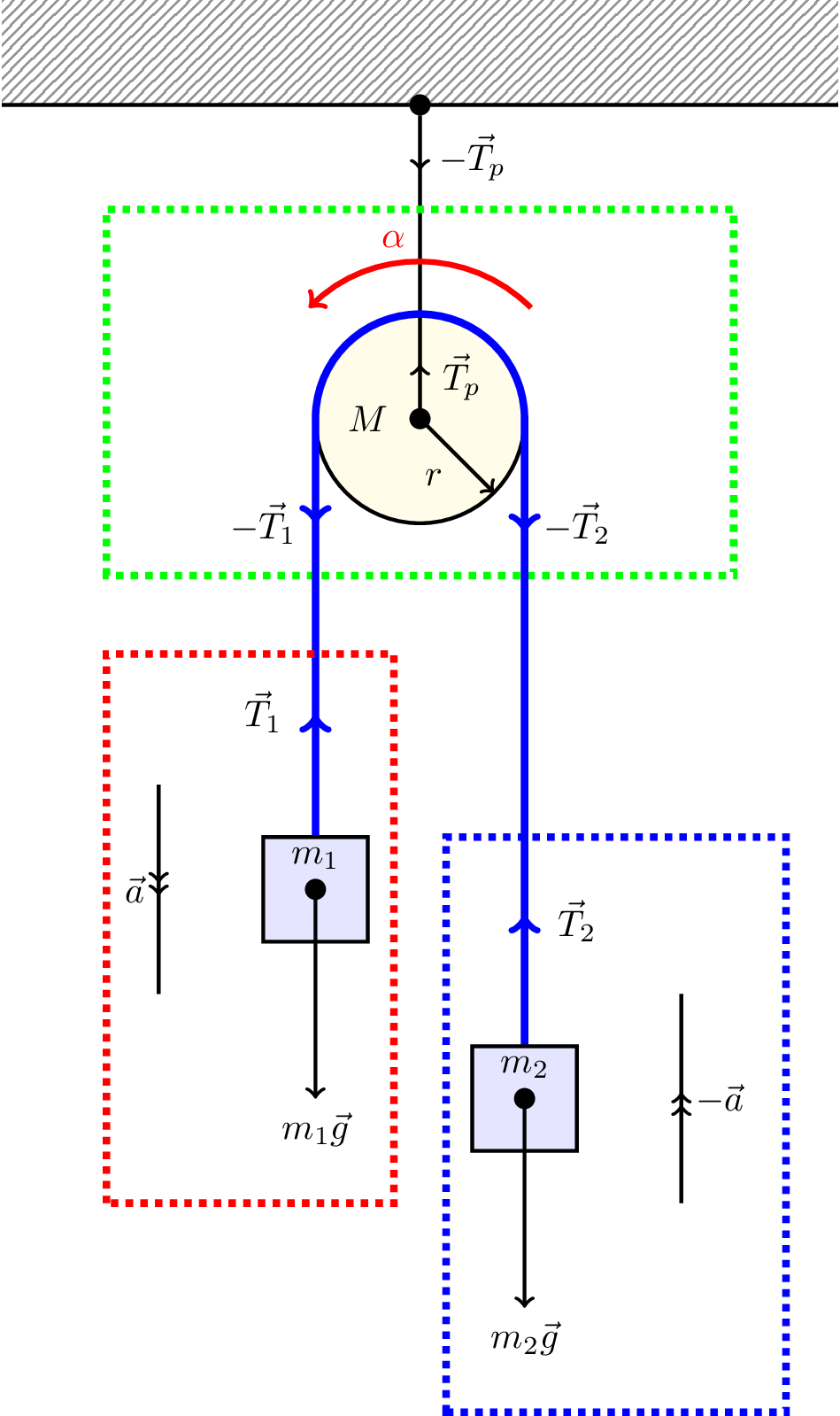
Let’s revisit the Atwood machine but now with a pulley that has some mass, and friction so that the rope does not slide over the pulley but causes it to rotate. We assume there is sufficient friction to stop the rope slipping over the pulley. The moment of inertia of the pulley is \(I = \beta Mr^2\) where \(\beta\) depends on the exact nature of the pulley (e.g., \(\beta = 1/2\) if the pulley is a solid disc). This is shown in Figure 8.12.
The angular acceleration of the pulley, \(\alpha\), is related to the linear acceleration \(|\vec{a}|\) by \[ \alpha = \frac{|\vec{a}|}{r} \] because the rope does not slip.
This friction also means that the tension is not the same on either side of the pulley, i.e., \(|\vec{T_1}| \ne |\vec{T_2}|\).
Let’s consider each part (outlined by dotted lines in Figure 8.12) separately.
Left hand weight (outlined in red): \[ m_1 g - T_1 = m_1 a \text{\hspace{24pt} (downwards)} \tag{8.8}\]
Right hand weight (outlined in blue): \[ T_2 - m_2 g = m_2 a \text{\hspace{24pt} (upwards)} \tag{8.9}\]
Pulley (outlined in green): Torque about the axis of the pulley (out of the page), anticlockwise is as follows \[ T_1 r - T_2 r = I \alpha = \beta M r^2 \frac{a}{r} \] \[ T_1 - T_2 = \beta M a \] From Equation 8.8 and Equation 8.9 we can write \[ T_1 = m_1 (a-g) \] \[ T_2 = m_2 (a+g) \] Therefore \[ m_1 (a-g) - m_2 (a+g) = \beta M a \] which rearranges to give \[ a = \frac{g(m_1 - m_2)}{m_1 + m_2 + \beta M} \]
This agrees with our previous result when \(M = 0\) (see Equation 7.1).
\(M > 0\) so in general acceleration lower than in case non massive pulley.
Let’s consider a cylinder (or ball), with moment of inertia \(I = \beta mr^2\), rolling down a slope without slipping, as shown in Figure 8.13.
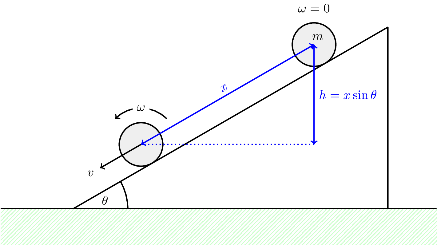
We assume the cylinder is not slipping so \[ v = r \omega \] and no work is done by friction.
We can consider conservation of energy to say \[ \text{PE lost} = \text{linear KE gained} + \text{rotational KE gained} \] \[ mgx\sin\theta = \frac{1}{2} mv^2 + \frac{1}{2} I \omega^2 \] \[ mgx\sin\theta = \frac{1}{2} mv^2 + \frac{1}{2} \beta mr^2 \left( \frac{v}{r} \right)^2 \] \[ v = \sqrt{\frac{2gx\sin\theta}{1 + \beta}} \]
The final speed depends on \(\beta\) and is larger for a sphere (\(\beta = 2/5\)) than a cylinder (\(\beta = 1/2\)).
Note: there is no dependence on mass only on \(\beta\), i.e., shape.