5 Fundamental Theorems
5.1 Fundamental Theorem of Calculus
\(f(x)\) is a function of one variable \[ \int_{a}^{b} \frac{d f}{d x} d x=f(b)-f(a) \] or \[ \int_{a}^{b} F(x) d x=f(b)-f(a), \]
where \(F(x)=\frac{d f}{d x}\). This tells you how to integrate \(F(x)\) - find a function \(f(x)\) with a derivate equal to \(F(x)\).
5.2 Fundamental Theorem of Gradients
For \(T(x, y, z)\) a scalar function and \(d T=\nabla T \cdot d \underline{l}\) \[ \int_{a}^{b} \nabla T \cdot d \ell=T(b)-T(a). \] In other words the line integral of the gradient is given by the value of the function at its boundaries.
Note: Gradients are special - the line integrals associated with them are path independent.
Lets check the Fundamental Theorem of Gradients assuming \(T = xy^2\) point \(a = (0,0,0)\) and \(b = (2, 1, 0)\).
We need to pick a path even though gradients are special and path independent. So lets take the path from point\(a\) to point \(b\) in two parts first horizonally along the x-axis (from \((0,0,0) \rightarrow (2, 0, 0)\)) and then vertically up to point \(b\) (\(\rightarrow (2,1,0)\)).
- Out along \(x\)-axis, \(d \underline{l}=dx \hat{x}+d y \hat{y}+d z \hat{z}\) \[ \begin{aligned} & \int_{i} \nabla T \cdot d \underline{l} \\ & d\underline{l} = dx\hat{x} \\ & \nabla T=y^{2} \hat{x}+2 x y \hat{y}, \quad y=0 \\ & \nabla T \cdot d l=0 \\ & \int_{i} \nabla T \cdot d l=0 \end{aligned} \]
- Now lets calculate the left hand side of the theorem for the second half of the path: \[ \begin{aligned} &\int_{i i} \nabla T \cdot d \underline{l}, \quad x=2\\ & \nabla T \cdot d \underline{l}=4 y d y \\ & \int_{0}^{1} 4 y d y=\left.2 y^{2}\right|_{0} ^{1}=2 \end{aligned} \]
Thus the entire integral is \(\int_{a}^{b} \nabla T \cdot d l=2\). Is this consistent with the fundamental theorem of gradients? Yes’ be cave \(T(b)-T(a)=2-0=2\).
Can check with another path.
- Lets take another path - the straight line from the origin to \((1, 2, 0)\) \[ \begin{aligned} y= 1 / 2 \, x, d y=1 / 2 \,d x \quad \nabla T \cdot d \underline{l} & =y^{2} d x+2 x y d y \\ & =\frac{1}{4} x^{2} d x+\frac{x^{2}}{2} d x \\ & =\frac{3}{4} x^{2} d x \\ \int_{\text {iii }}^{2} \nabla \cdot d \underline{l}=\int_{0}^{2} \frac{3}{4} x^{2} d x=\left.\frac{1}{4} x^{3}\right|_{0} ^{2}= 2 & \end{aligned} \]
5.3 Fundamental Theorem of Divergence
\[ \int_{V}(\nabla \cdot \underline{v}) d T=\oint_{S} \underline{v} \cdot d \underline{a} \]
This is saying that the integral of the derivative (divergence) over a region (volume) is equal to the value at of the function at the boundary (at the bounding surface of the volume). This is also called Gauss’s Theorem \(\Rightarrow\) super useful in electrodynamics.
The divergence represents the “spreading out” so if \(\underline{v}\) represents the flow of incompressible fluid then the right hand side is the flux through the surface \[ \int \text { faucets within the volume }=\oint \begin{gathered} \text { flow out through } \\ \text { the surface } \end{gathered} \]
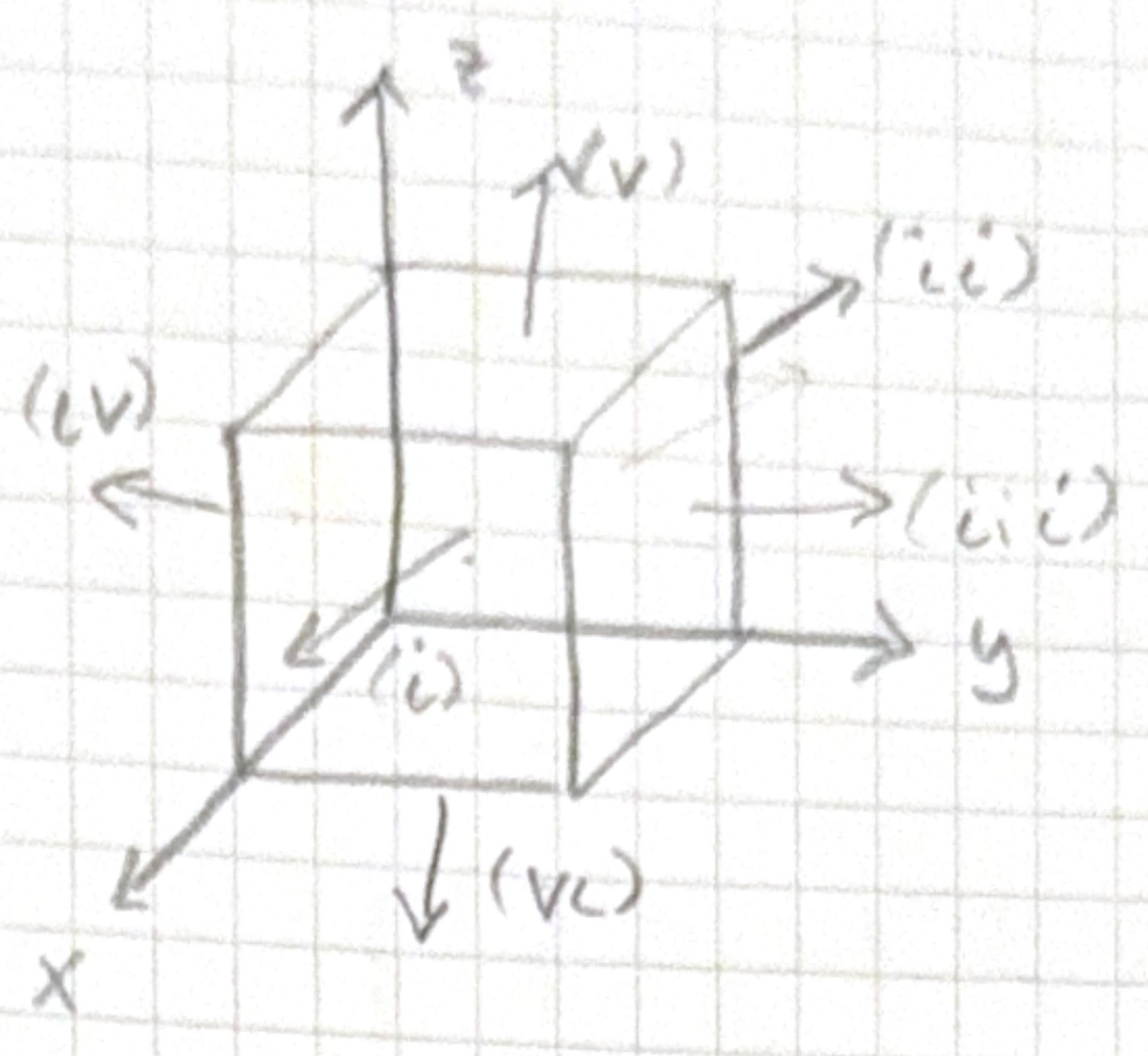
Check the divergence theorem
\[ \underline{v}=y^{2} \hat{x}+\left(2 x y+z^{2}\right) \hat{y}+2 y z \hat{z} \] and a unit cube placed at the origin
\[ \begin{aligned} & \nabla \cdot \underline{v}=0+2 x+2 y \\ & \int_{V} 2(x+y) d \tau=\int_{0}^{1} \int_{0}^{1} \int_{0}^{1} 2(x+y) d x d y d z \\ & =\left.2 \int_{0}^{1} \int_{0}^{1}\left(\frac{x^{2}}{2}+y x\right)\right|_{0} ^{1} d y d z \\ & =2 \int_{0}^{1} \int_{0}^{1}(1 / 2+y) d y d z \\ & =\left.2 \int_{0}^{1} d z\left(1 / 2 y+1 / 2 y^{2}\right)\right|_{0} ^{1} \\ & =2(1 / 2+1 / 2)=2 \text {. } \end{aligned} \]
Left side of the divergence theorem. \(\oint_{S} \underline{v} \cdot d \underline{a}\) (right side) \(\Rightarrow\) consider each side:
Side 1: \(x=1\) and \(d \underline{a}=d y d z \hat{x}\) \[ \begin{aligned} \underline{v} \cdot d \underline{a} & =y^{2} d y d z \\ \int_{\text {side 1}} \underline{v} \cdot d \underline{a}=\int_{0}^{1} \int_{0}^{1} y^{2} d y d z & =\left.\int_{0}^{1} \frac{y^{3}}{3}\right|_{0} ^{1} d z \\ & =\frac{1}{3} \end{aligned} \]
Side 2: \(x=0 \quad d a=-d y d z \hat{x}\) \[ \int_{\text {side } 2} y \cdot d \underline{a}=-\int_{0}^{1} \int_{0}^{1} y^{2} d y d z=-\frac{1}{3} . \]
Side 3: \(y=1 \quad d \underline{a}=d x d z \hat{y}\) \[ \begin{aligned} \int_{\text {side } 3} \underline{v} \cdot d \underline{a} & =\int_{0}^{1} \int_{0}^{1} 2 x y+z^{2} d x d z \\ & =\int_{0}^{1} \int_{0}^{1}\left(2 x+z^{2}\right) d x d z \\ & =\left.\int_{0}^{1}\left(x^{2}+x z^{2}\right)\right|_{0} ^{1} d z \\ & =\int_{0}^{1} 1+z^{2} d z \\ & =z+\left.\frac{z^{3}}{3}\right|_{0} ^{1} \\ & =\frac{4}{3} . \end{aligned} \]
Side 4: \(y=0 \quad d \underline{a}=-d x d z \hat{y}\) \[ \begin{aligned} \int_{\text {side 4}} \underline{v} \cdot d \underline{a} & =-\int_{0}^{1} \int_{0}^{1} z^{2} d y d z \\ & =-\int_{0}^{1} z^{2} d z \\ & =-\frac{1}{3} \cdot \end{aligned} \]
Side 5: \(z=1 \quad d \underline{a}=d x d y \hat{z}\) \[ \begin{aligned} \int_{side 5} \underline{v} \cdot d \underline{a} & =\int_{0}^{1} \int_{0}^{1} 2 y d x d y \\ & =\int_{0}^{1} 2 y d y=1 . \end{aligned} \] side 6: \(z = 0 \quad d \underline{a}=-d x d y \hat{z}\) \[ \begin{aligned} \int_{side 6} \underline{v} \cdot d \underline{a}= & -\int_{0}^{1} \int_{0}^{1} 0 d x d y=0 \\ \therefore \oint_{S} \underline{v} \cdot d \underline{a} & =\frac{1}{3}-\frac{1}{3}+\frac{4}{3}-\frac{1}{3}+1+0 \\ & =2 \end{aligned} \]
5.4 Fundamental Theorem of Curls
\[ \int_{S}(\nabla \times \underline{v}) \cdot d \underline{a} =\oint_{P} \underline{v} \cdot d \underline{l} \]
The integral of a derivative (curl) over a region (patch of surface) equals the value at the boundary (path). This is also called Stokes Theorem.
The left side depends only on the boundary line not the surface used.
Note: For a closed surface
\[ \oint_{S}(\nabla \times \underline{v}) \cdot d \underline{a} =0. \]
Check Stokes theorem - \(\underline{v}=\left(2 x z+y^2\right) \hat{y}+\left(4 y z^{2}\right) \hat{z}\).
\[ \begin{aligned} & \nabla \times \underline{v}=\left|\begin{array}{ccc} \hat{x} & \hat{y} & \hat{z} \\ \partial / \partial x & \partial / \partial y & \partial / \partial z \\ 0 & 2 x z+3 y^{2} & 4 y z^{2} \end{array}\right| \\ &=\hat{x}\left(\frac{\partial 4 y z^{2}}{\partial y}-\frac{\partial}{\partial z}\left(2 x z+3 y^{2}\right)\right) \\ &-\hat{y}\left(\frac{\partial}{\partial x} 4 y z^{2}-\frac{\partial 0}{\partial z}\right) \\ &+\hat{z}\left(\frac{\partial}{\partial x}\left(2 x z+3 y^{2}\right)-\frac{\partial}{\partial y}(0)\right) \\ &=\hat{x}\left(4 z^{2}-2 x\right)-\hat{y}(0)+\hat{z}(2 x) \\ &=\left(4 z^{2}-2 x\right) \hat{x}+2 x \hat{z} \\ & d \underline{a}=d y d z \hat{x}, x=0,(\nabla \times \underline{v}) \cdot d \underline{a}=\left(4 z^{2}-2 x\right) \hat{x} \cdot d y d z \hat{x} \\ & =\left(4 z^{2}-2 x\right) d y d z \\ & \int \nabla \times \underline{v} \cdot d \underline{a} = \int_{0}^{1} \int_{0}^{1}\left(4 z^{2}-2 x\right) d y d z \\ &=\int_{0}^{1} \int_{0}^{1} 4 z^{2} d y d z \\ &=\int_{0}^{1} 4 z^{2} d z=4 / 3 . \end{aligned} \]
Ok so now lets try the path side
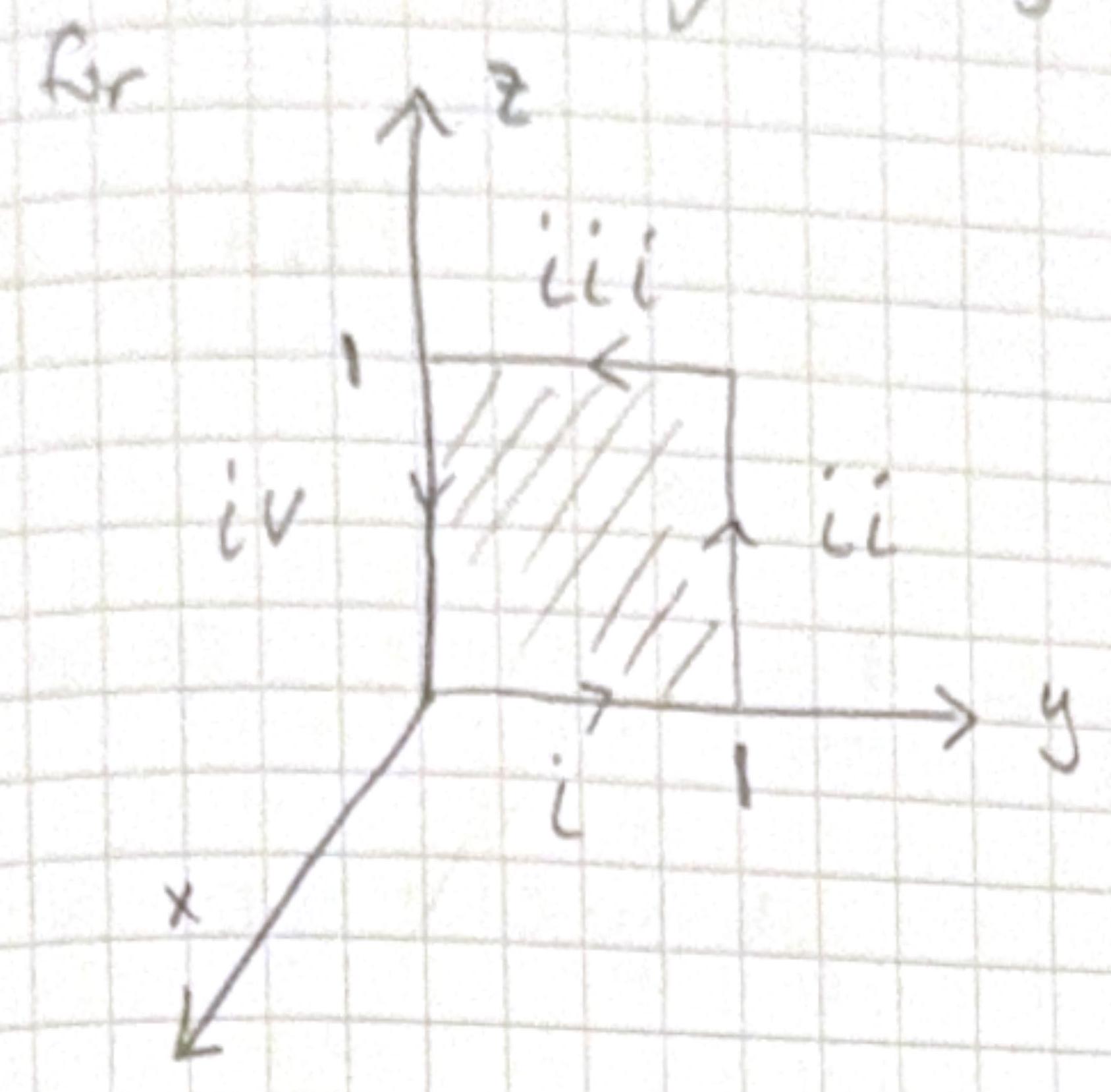
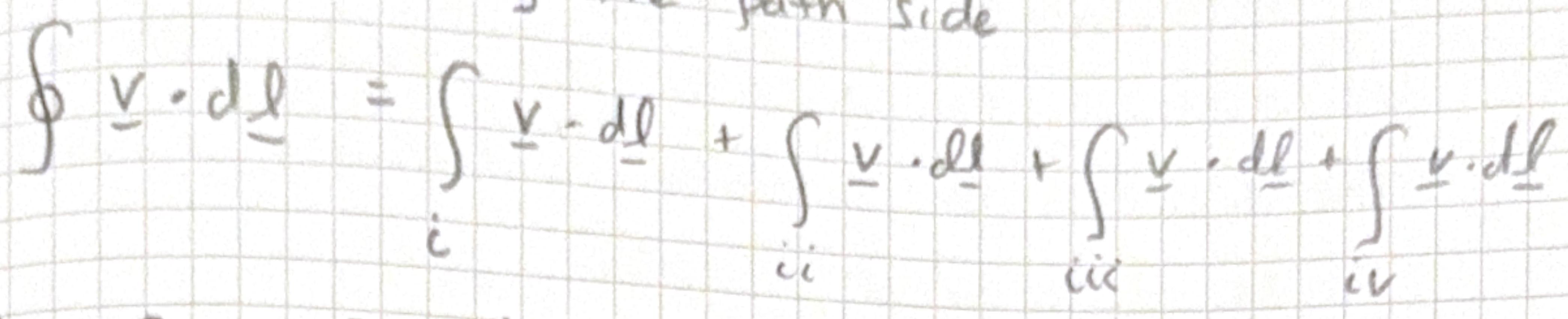
Part i \[ \begin{aligned} & x=0, z=0, \quad d \underline{l}=d y \hat{y} \\ & \underline{v} \cdot d \underline{l}=3 y^{2} d y \quad \quad \int_{i} \underline{v} \cdot d \underline{l}=\int_{0}^{1} 3 y^{2} d y=1 \end{aligned} \]
Part ii \[ \begin{aligned} & y=1, x=0, d \underline{l}=d z \hat{z} \\ & \underline{v} \cdot d \underline{l}=4 y z^{2} d z=4 z^{2} d z \\ & \int_{i i} \underline{v} \cdot d \underline{l}=\int_{0}^{1} 4 z^{2} d z=\frac{4}{3}. \end{aligned} \]
Part iii \[ \begin{aligned} & x=0, z=1, d \underline{l}=-d y \hat{y} \\ & \underline{v} \cdot d \underline{l}=-\left(2 x z+3 y^{2}\right) d y=-3 y^{2} d y \\ & \int_{i i i} \underline{v} \cdot d \underline{l}=\int_{1}^{0} 3 y^{2} d y=\left.y^{3}\right|_{1} ^{0}=-1 \end{aligned} \] Part iv \[ \begin{aligned} & x=0, y=0 \quad d \underline{l}=-d z \hat{z} \\ & \underline{v} \cdot d \underline{l}= - 4 y z^{2} d z=0 . \\ & \int_{iv} \underline{v} \cdot d \underline{l}=\int_{1}^{0} 0 d z=0 \\ & \oint v \cdot d \underline{l}=1+4 / 3-1+0 =4 / 3 \end{aligned} \]